Inside the Oracle BI Server Part 2 : How Is A Query Processed?

In the first article on this series about the Oracle BI Server, I looked at the architecture and functions within this core part of the OBIEE product set. in this article, I want to look closer at what happens when a query (or "request") comes into the BI Server, and how it translates it into the SQL, MDX, file and XML requests that then get passed to the underlying data sources.

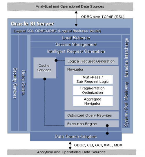
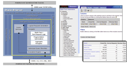
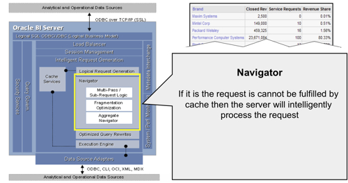
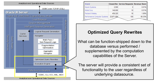
In the previous article, I laid out a conceptual diagram of the BI Server and talked about how the Navigator turned incoming queries into one or more physical database queries. As a recap, here's the architecture diagram again:

Bis2-1

Now as we all know, the BI Server uses a three-layer metadata model that exposes one or more databases (or "subject areas") for ODBC-compliant query tools to run queries against. Here's a typical metadata model that takes a number of physical data sources, joins them together into a smaller number of business model and mapping models, and then presents them out to the query tool (usually, Oracle BI Answers) as a set of databases made up of relational tables, columns and joins.

Bis7

Usually you access this metadata model using Oracle BI Answers, which presents you with an initial choice of subject areas (databases in ODBC terminology) and then displays the contents of one of them as a list of tables and columns (in 11g, you'll be able to to include tables from multiple subject areas in queries as long as there are tables in common between them).

Bis9

Other ODBC-compliant query tools, such as Microsoft Excel, Cognos or Business Objects, can access these subject areas and run queries against them just as if it was a regular database. Here's Microsoft Excel 2007 building a query against the same subject area:

Bis8

What Happens When the BI Server Handles a Query? So just what happens then, when a query (or "request') comes in from one of these sources, and needs to be processed in order to return results to the user? As you're probably aware, the BI Server doesn't itself hold data (except cached results from other queries, when this feature is enabled); instead, it translates the incoming "logical" query into one or more outgoing "physical" queries against the relevant data sources. As such, a logical model presented to users might be mapped to data in an Oracle data warehouse, an E-Business Suite application, some data in a Teradata data warehouse, some measures in an Essbase cube and even some data in an Excel spreadsheet. The BI server resolves this complexity by creating a simplified, star schema business model over these data sources so that the user can query it as if it's a single source of data.

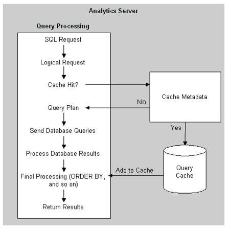
If you're used to the Oracle database, you'll probably know that it has various components that are used to resolve queries - the library cache, query rewrite, table and system statistics, etc - and both rule-based and cost-based optimizers that are used to generate a query plan. For most modern Oracle systems, a statistics-based cost-based optimizer (most famously documented by Jonathan Lewis in this book) is used to generate a number of potential execution plans (which can be displayed in a 10035 trace), with the lowest cost being chosen to run the query. Now whilst the equivalent process isn't really documented for the BI Server, what it appears to do is largely follow a rule-based approach with a small amount of statistics being used (or not used, as I'll mention in a moment). In essence, the following sources of metadata information are consulted when creating the query plan for the BI Server;

  • The presentation (subject area) layer to business model layer mapping rules;
  • The logical table sources for each of the business columns used in the request;
  • The dimension level mappings for each of the logical table sources;
  • The "Number of Elements at this Level" count for each dimension level (potentially the statistics bit, though anecdotally I've heard that these figures aren't actually used by the BI Server);
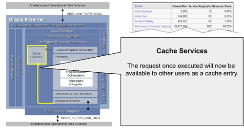
  • Whether caching is enabled, and if so, whether the query can be found in the cache;
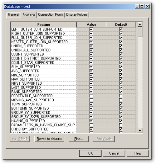
  • What physical features are enabled for the particular source database for each column (and whether they are relational, multi-dimensional, file, XML or whatever)
  • Specific rules for generating time-series queries, binning etc, and
  • Security settings and filters
As far as I can tell, there are no indexes, no statistics (apart from the dimension level statistics mentioned above) and no hints; there is however query rewrite and aggregates, as the BI Server allows aggregate tables to be defined which are then mapped in to specific levels in a dimension hierarchy. Cleverly, the back-end data source doesn't even have to be an SQL database, and can in fact be a multi-dimensional database such as Essbase, Oracle OLAP or Microsoft Analysis Services, with the multi-dimensional dataset that they return converted into a row-based dataset that can be joined to other data coming in from a more traditional relational database.

"A Day in the Life of a Query"

A good way of looking at what Oracle has termed "A day in the life of a query", is to take a look at some slides from a presentation that Oracle used regularly around the time of the introduction of Oracle BI EE. I'll go through it slide by slide and add some interpretation from myself.

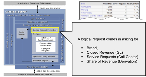
  1. A query comes in from Answers or any other ODBC query tool, asking for one or more columns from a subject area. Overall, the function within the BI Server that deals with this is called Intelligent Request Generation, marked in yellow in the diagram below.

Bis10

2. The query is then passed to the Logical Request Generation engine, marked in yellow in the diagram below. The request itself requires the Brand, Closed Revenue (ultimately held in the GL system), Service Requests (held in the CRM system) and Share of Revenue (a calculated, or derived, measure). As such it's going to require multiple physical SQL queries and multi-pass calculations, all of which will be worked out by another part of the BI Server architecture, the Navigator.

Bis11

3. Once the logical request has been generated but before its passed off to the Navigator, a check is made (if this feature is enabled) as to whether the logical request can be found in the cache. Cache Services will either do a fast, or more comprehensive match of the incoming request against those stored in the query cache, and if found, return the results from there rather than have the BI Server run physical SQL against the business model's data sources.

Bis12

For a more detailed look at what Cache Services does, the old Siebel Analytics Administration Tool documentation has a good flowchart that explains what goes on:

Bis13

The key bit is the Cache Hit step. In general, a cache hit will occur if the following conditions are met:
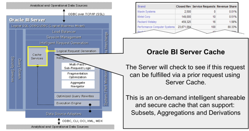
  • Caching is enabled (CACHE=Y in the NQSConfig.INI file);
  • The WHERE clause in the logical SQL is semantically the same, or a logical subset of a cached statement;
  • All of the columns in the SELECT list have to exist in the cached query, or they must be able to be calculated from them;
  • It has equivalent join conditions, so that the resultant joined table of any incoming query has to be the same as (or a subset of) the cached results
  • If DISTINCT is used, the cached copy has to use this attribute as well
  • Aggregation levels have to be compatible, being either the same or more aggregated than the cached query
  • No further aggregation (for example, RANK) can be used in the incoming query
  • Any ORDER BY clause has to use columns that are also in the cached SELECT list
In addition, there are two NQSConfig.INI parameters that I think were added in the last few releases (as I can't find them mentioned in the Siebel Analytics documentation) are USE_ADVANCED_HIT_DETECTION and MAX_SUBEXPR_SEARCH_DEPTH. The latter determines how many levels into an expression (for example, SUM(MAX(SIN(COS(TAN(ABS(TRUNC(PROFIT)))))))) that the cache hit detector will go in trying to get a match, whilst the former turns on some additional cache hit searches that you might want to enable if caching is important but not otherwise happening. Unfortunately the docs don't really expand on what these additional searches are or the performance impact that they can introduce, so if anyone has any more information on this, I'd be glad to hear.
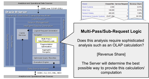
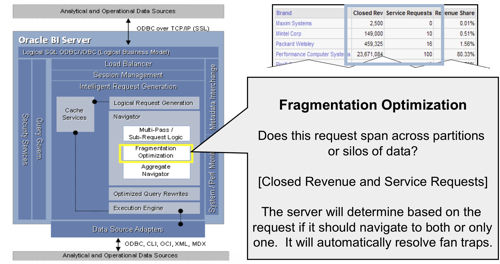
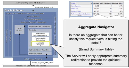
  1. If the cache can't provide the answer to the request, the request then gets passed to the Navigator. The Navigator handles the logical request "decision tree" and determines how complex the request is, what data sources (logical table sources) need to be used, whether there are any aggregates that can be used, and overall what is the best way to satisfy the request, based on how you've set up the presentation, business model and mapping, and physical layers in your RPD.

Bis14

5. Within the Navigator, the Multi-Pass / Sub-Request Logic function analyzes the incoming request and works out the complexity of the query. It works out whether it requires multiple passes (for example, calculates the average of two aggregated measures), or whether the request is based on the results of another request (in other words, uses a sub-request). The BI Server then uses this information to work out the optimal way to gather the required data and do the calculations; in the example used in the slides, the revenue share calculation is based on the other two measures and is therefore considered "multi-pass".

Bis15

6. A measure used within the business model and mapping layer may be "fragmented", which means that it is logically partitioned so that historic information, for examples, comes from a data warehouse whilst current information comes from an OLTP application. The Fragment Optimization Engine within the Navigator sits between the incoming request and the Execution Engine and where appropriate, transforms the base-level SQL into "fragmented" SQL against each of the data sources mapped into the fragmented measure. For more background information on fragmentation, check out this old blog post on the subject.

Bis17

7. The final function within the Navigator is the Aggregate Navigator, which uses the logical table source mappings together (in theory) with the dimension level statistics to determine the most efficient table to fetch the data from (i.e. the table with the least number of records to successfully fulfil a request).

Bis16

8. The Optimized Query Rewrites function within the BI Server then takes the query plan generated by the Navigator and rewrites it to use the features of the underlying database engines, adding RANK(OVER()) calculations if Oracle is being used, for example (referred to as "function shipping") or just getting the raw data and having the BI Server do the calculations afterwards, if working with a database that doesn't support analytic SQL functions. This part of the BI Server is also responsible for generating XML queries, or MDX queries for OLAP sources, which are then sent to the underlying physical databases, in parallel, so that they can retrieve their relevant data sets.

Bis18

9. Once the data is retrieved, the results combined together and any further calculations applied, the results are returned to the calling application via the ODBC interface, and also copied to the cache along with the logical SQL query if caching is enabled.

Bis21

The BI Server's knowledge of what each source database can support, in terms of SQL functions, is determined by the contents of the DBFeatures.INI configuration file which can in turn be over-ridden by the "Features" tab in the Database settings in the physical database model.

Bis19

I think I've also noticed that, from release to release of OBIEE, the way that time-series queries, for example, get resolved into physical SQL queries changes over time, as Oracle get better at generating efficient SQL queries to resolve complex calculations. It's also the case that currently, for Essbase data sources, very few of the functions used by the BI Server get function-shipped to their equivalent MDX functions, though this is meant to be improving in the forthcoming 11g release (and in the meantime, you can use EVALUATE and EVALUATE_AGGR to call MDX functions directly).

Level 5 Logging, and Logical Execution Plans

You can see what goes on when a complex, multi-pass request that requires multiple data sources is sent through from Answers and gets logged in the NQQuery.log file with level 5 logging enabled. The query requests "quantity" information that is held in an Oracle database, "quotas" that comes from an Excel spreadsheet, and "variance" which is derived from quantity minus quotas. Both columns need to be aggregated before the variance calculation can take place, and you can see from the logs the Navigator being used to resolve the query.

Starting off, this is the logical request coming through.

-------------------- Logical Request (before navigation):

RqList
    Times.Month Name as c1 GB,
    Quantity:[DAggr(Items.Quantity by [ Times.Month Name, Times.Month ID] )] as c2 GB,
    Quota:[DAggr(Items.Quota by [ Times.Month Name, Times.Month ID] )] as c3 GB,
    Quantity:[DAggr(Items.Quantity by [ Times.Month Name, Times.Month ID] )] - Quota:[DAggr(Items.Quota by [ Times.Month Name, Times.Month ID] )] as c4 GB,
    Times.Month ID as c5 GB
OrderBy: c5 asc
Then the navigator breaks the query down, works out what sources, multi-pass calculations and aggregates can be used, and generates the logical query plan.
-------------------- Execution plan:

RqList <<993147>> [for database 0:0,0]
    D1.c1 as c1 [for database 0:0,0],
    D1.c2 as c2 [for database 3023:491167,44],
    D1.c3 as c3 [for database 0:0,0],
    D1.c4 as c4 [for database 0:0,0]
Child Nodes (RqJoinSpec): <<993160>> [for database 0:0,0]
    (
        RqList <<993129>> [for database 0:0,0]
            D1.c1 as c1 [for database 0:0,0],
            D1.c2 as c2 [for database 3023:491167,44],
            D1.c3 as c3 [for database 0:0,0],
            D1.c4 as c4 [for database 0:0,0],
            D1.c5 as c5 [for database 0:0,0]
        Child Nodes (RqJoinSpec): <<993144>> [for database 0:0,0]
            (
                RqBreakFilter <<993128>>[1,5] [for database 0:0,0]
                    RqList <<992997>> [for database 0:0,0]
                        case  when D903.c1 is not null then D903.c1 when D903.c2 is not null then D903.c2 end  as c1 GB [for database 0:0,0],
                        D903.c3 as c2 GB [for database 3023:491167,44],
                        D903.c4 as c3 GB [for database 0:0,0],
                        D903.c3 - D903.c4 as c4 GB [for database 0:0,0],
                        case  when D903.c5 is not null then D903.c5 when D903.c6 is not null then D903.c6 end  as c5 GB [for database 0:0,0]
                    Child Nodes (RqJoinSpec): <<993162>> [for database 0:0,0]
                        (
                            RqList <<993219>> [for database 0:0,0]
                                D902.c1 as c1 [for database 0:0,0],
                                D901.c1 as c2 [for database 3023:491167,44],
                                D901.c2 as c3 GB [for database 3023:491167,44],
                                D902.c2 as c4 GB [for database 0:0,0],
                                D902.c3 as c5 [for database 0:0,0],
                                D901.c3 as c6 [for database 3023:491167,44]
                            Child Nodes (RqJoinSpec): <<993222>> [for database 0:0,0]

                                    (
                                        RqList <<993168>> [for database 3023:491167:ORCL,44]
                                            D1.c2 as c1 [for database 3023:491167,44],
                                            D1.c1 as c2 GB [for database 3023:491167,44],
                                            D1.c3 as c3 [for database 3023:491167,44]
                                        Child Nodes (RqJoinSpec): <<993171>> [for database 3023:491167:ORCL,44]
                                            (
                                                RqBreakFilter <<993051>>[2] [for database 3023:491167:ORCL,44]
                                                    RqList <<993263>> [for database 3023:491167:ORCL,44]
                                                        sum(ITEMS.QUANTITY by [ TIMES.MONTH_MON_YYYY] ) as c1 [for database 3023:491167,44],
                                                        TIMES.MONTH_MON_YYYY as c2 [for database 3023:491167,44],
                                                        TIMES.MONTH_YYYYMM as c3 [for database 3023:491167,44]
                                                    Child Nodes (RqJoinSpec): <<993047>> [for database 3023:491167:ORCL,44]
                                                        TIMES T492004
                                                        ITEMS T491980
                                                        ORDERS T491989
                                                    DetailFilter: ITEMS.ORDID = ORDERS.ORDID and ORDERS.ORDERDATE = TIMES.DAY_ID [for database 0:0]
                                                    GroupBy: [ TIMES.MONTH_MON_YYYY, TIMES.MONTH_YYYYMM]  [for database 3023:491167,44]
                                            ) as D1
                                        OrderBy: c1 asc [for database 3023:491167,44]
                                    ) as D901 FullOuterStitchJoin <<993122>> On D901.c1 =NullsEqual D902.c1; actual join vectors:  [ 0 ] =  [ 0 ]

                                    (
                                        RqList <<993192>> [for database 0:0,0]
                                            D2.c2 as c1 [for database 0:0,0],
                                            D2.c1 as c2 GB [for database 0:0,0],
                                            D2.c3 as c3 [for database 0:0,0]
                                        Child Nodes (RqJoinSpec): <<993195>> [for database 0:0,0]
                                            (
                                                RqBreakFilter <<993093>>[2] [for database 0:0,0]
                                                    RqList <<993319>> [for database 0:0,0]
                                                        D1.c1 as c1 [for database 0:0,0],
                                                        D1.c2 as c2 [for database 0:0,0],
                                                        D1.c3 as c3 [for database 0:0,0]
                                                    Child Nodes (RqJoinSpec): <<993334>> [for database 0:0,0]
                                                        (
                                                            RqList <<993278>> [for database 3023:496360:Quotas,2]
                                                                sum(QUANTITY_QUOTAS.QUOTA by [ MONTHS.MONTH_MON_YYYY] ) as c1 [for database 3023:496360,2],
                                                                MONTHS.MONTH_MON_YYYY as c2 [for database 3023:496360,2],
                                                                MONTHS.MONTH_YYYYMM as c3 [for database 3023:496360,2]
                                                            Child Nodes (RqJoinSpec): <<993089>> [for database 3023:496360:Quotas,2]
                                                                MONTHS T496365
                                                                QUANTITY_QUOTAS T496369
                                                            DetailFilter: MONTHS.MONTH_YYYYMM = QUANTITY_QUOTAS.MONTH_YYYYMM [for database 0:0]
                                                            GroupBy: [ MONTHS.MONTH_YYYYMM, MONTHS.MONTH_MON_YYYY]  [for database 3023:496360,2]
                                                        ) as D1
                                                    OrderBy: c2 [for database 0:0,0]
                                            ) as D2
                                        OrderBy: c1 asc [for database 0:0,0]
                                    ) as D902
                        ) as D903
                    OrderBy: c1, c5 [for database 0:0,0]
            ) as D1
        OrderBy: c5 asc [for database 0:0,0]
    ) as D1
Notice the "FullOuterStitchJoin" in the middle of the plan? We'll look into this more in the next posting in this series. For now though, this logical query plan is then passed to the Optimized Query Rewrites and Execution Engine, which then generates in this case two physical SQL statements that are then passed back, and "stitch joined", by the BI Server, before performing the post-aggregation calculation required for the variance measure.
-------------------- Sending query to database named ORCL (id: <<993168>>):

select D1.c2 as c1,
     D1.c1 as c2,
     D1.c3 as c3
from
     (select D1.c1 as c1,
               D1.c2 as c2,
               D1.c3 as c3
          from
               (select sum(T491980.QUANTITY) as c1,
                         T492004.MONTH_MON_YYYY as c2,
                         T492004.MONTH_YYYYMM as c3,
                         ROW_NUMBER() OVER (PARTITION BY T492004.MONTH_MON_YYYY ORDER BY T492004.MONTH_MON_YYYY ASC) as c4
                    from
                         CUST_ORDER_HISTORY.TIMES T492004,
                         CUST_ORDER_HISTORY.ITEMS T491980,
                         CUST_ORDER_HISTORY.ORDERS T491989
                    where  ( T491980.ORDID = T491989.ORDID and T491989.ORDERDATE = T492004.DAY_ID )
                    group by T492004.MONTH_MON_YYYY, T492004.MONTH_YYYYMM
               ) D1
          where  ( D1.c4 = 1 )
     ) D1
order by c1


+++Administrator:2b0000:2b000e:----2010/02/23 16:04:42

-------------------- Sending query to database named Quotas (id: <<993278>>):
select sum(T496369."QUOTA") as c1,
     T496365."MONTH_MON_YYYY" as c2,
     T496365."MONTH_YYYYMM" as c3
from
     "MONTHS" T496365,
     "QUANTITY_QUOTAS" T496369
where  ( T496365."MONTH_YYYYMM" = T496369."MONTH_YYYYMM" )
group by T496365."MONTH_YYYYMM", T496365."MONTH_MON_YYYY"

Memory Usage and Paging Files

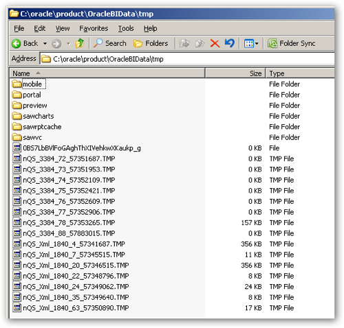
If you follow the BI Server at the process level during these steps, you'll find that memory usage is largely determined at startup time by the size and complexity of the RPD thats attached online, and then goes up by around 50MB when the first query is executed. After that, memory usage tends to go up the more concurrent sessions that are run, and also when cross-database joins are performed. You'll also find TMP files being created in $ORACLEBIDATA/tmp directory, which are used by the BI Server to hold temporary data as it pages out from memory, again typically when cross-database joins are used but also when it needs to perform additional aggregations that can't be put into the physical SQL query.

Bis20

These files can get fairly big (up to 2GB in some cases) and can be created even when a single data source is used, typically for grouping data or as we'll see in the next posting, when joining data across fact tables. They are usually cleared down when the BI Server and Presentation Server are restarted, but bear in mind when creating complex calculations that they can get pretty I/O intensive on the BI Server hardware.

So that's the basics in terms of how basic queries are processed by the BI Server, and how the various BI Server components and engines process the query as it goes through the various stages. Again, if anyone knows any more, please add it as a comment, but for now that's it and I'll be back in a few days with part 3, on BI Server In-Memory Joins.