Using OBIEE against Transactional Schemas Part 3: Simple Dimensions and Facts

This could be the longest series of blog posts in Rittman Mead history... not in number of posts (this is only the third), but in length of time from start to finish. I don't think that's a record anyone is actively pursuing, nor am I proud to (possibly) be the record holder, so my apologies to those of you waiting anxiously for each new installment. To reset... I'm discussing using OBIEE to report against transactional schemas. I started with an introduction, and followed up with a few words on aliases. Now I'd like to discuss a general approach to defining logical fact and dimensional tables in the OBIEE Business Model and Mapping layer.

Finding logical tables buried away in a highly normalized model is really as simple as taking a business view of the data. With Customer data for instance, business users don’t think about (or even understand) normalized models with separate entities for Customer, and Customer Category, and Customer Type, and Customer Status, etc. To the business users, these are all attributes of a single entity: Customer. If we think about the BMM layer in OBIEE as a way to present a uniformed model to a business user, or at least a basic user with no knowledge of the underlying 3NF model used for running the business, then we should ask ourselves a simple question: how would a business user want to see this data?

So our job is to undo the brilliant normalization work performed by the transactional data modelers, and combine all of these separate entities into a single, conformed dimension table or fact table. In it’s purest form, I am describing nothing more than real-time ETL, because the logic applied in the BMM is the same sort of logic we would use in an ETL tool to construct facts and dimensions in the physical world.

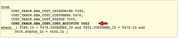
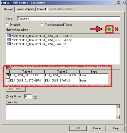
Thinking only about logical dimension tables for a moment, we start with the most basic and granular entity that composes the heart of the logical dimension, and start joining outward to include all the other ancillary entities needed to form a complete picture of that dimension. With the Customer Tracking application, the logical place to start is the Dim - Customer logical dimension, and the most basic table to use as a starting point is EBA_CUST_CUSTOMERS. This table contains the main attributes of Customer: the name, the address, etc. So I’ll construct a logical table source and start with the EBA_CUST_CUSTOMERS table, and then I’ll add additional physical entities using the (+) button, as depicted below.

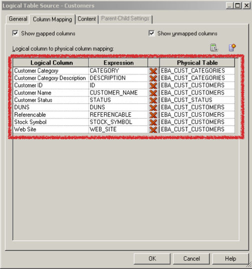
Once we have all the required tables joined into the logical table source, we can start mapping the physical columns to our desired logical columns, using either the Column Mapping tab in the logical table source, or by simply clicking and dragging physical columns over onto the logical dimension table.

Once all the columns have been mapped to one of the entities in our logical table source, we can then start building the hierarchy, or dimension in OBIEE terms, that defines the relationship among levels in the dimension. When we are reporting against a pure star schema, this kind of information doesn’t exist in the table definition, though hopefully it exists in the project documentation. However, when reporting off a transactional schema, we have a leg-up here. Although our logical dimension table presents as a single, conformed entity, our physical model is still 3NF, and a 3NF model gives us some hints regarding hierarchies, as those relationships are usually normalized out into separate tables. All and all, the process of building the hierarchy is no different from pure star schemas, because the logical dimension table shields us from the complexity of navigating multiple physical tables to define our hierarchy.

Shifting gears for a moment and thinking about fact tables, the process for mapping simple logical fact tables is at it's core very similar to the process for logical dimensional tables. When our source system has transactional data, with many measures, such as transaction amount, transaction quantity, etc., then defining the fact table is relatively simple, even though the logical table source for the logical fact table may contain a join across multiple source entities, similar to how we built the simple dimension table above. A common scenario for this is with a Sales Order, where these is a Sales Order Detail table and a Sales Order Header table.

The first approach I want to demonstrate is not as easy as the Sales Order example; it involves a more operational reporting requirement, and how to arrange our logical fact table when we really have no measures at all. In this scenario, what we have is a sort of relationship table, where we require a fact table, but the purpose of that fact table is only to form a bridge between various dimensional tables. Ralph Kimball calls this form of relationship table a factless fact table. As Kimball explains, the event is the fact, and he uses the example of the student attendance fact, where the only thing that is being recorded in the fact is the presence of a particular student, in a particular class, with a particular professor, on a particular day, etc. For the Customer Tracking application, we want to report on customer activities stored in the EBA_CUST_CUST_ACTIVITY table:

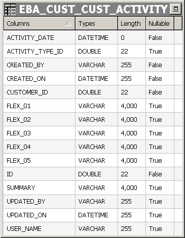
This table stores our basic CRM events: phone calls, meetings, delivered proposals, etc. But true to Kimball’s positioning of our requirement, this table doesn’t have any explicit facts such as amount sold, quantity sold, etc. We need a way to model these activities in the semantic layer in a way that makes sense to the BI Server, and what makes sense to the BI Server is the presence of at least one measure. This measure is required to provide the BI Server with the ability to generate aggregate queries involving SUM, AVG, etc. When we build a factless fact table in a data warehouse, we typically load each row with the appropriate surrogate keys to the dimension tables, along with a single, manufactured measure which is usually a value of 1.

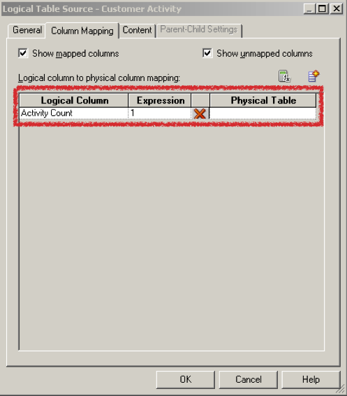
We use this value as the activity count, and we can use the measure as a basis for aggregate functions across different dimensions of the data. In building a logical factless fact table, we need to do the same thing. So we start with a logical source for the fact table, even though it doesn’t have any actual measures we will use. In the case of the Customer Tracking application, our relationship table, or factless fact, will be based on EBA_CUST_CUST_ACTIVTY, which is a table with a single record for each activity that we want to record for a customer. Once we have defined the physical table for our logical table source, we map the source column for the Activity Count measure, which in our case will always be a value of 1:

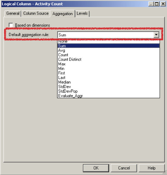
Once we have the new "fake" measure, we can set the aggregation rule, in this case SUM:

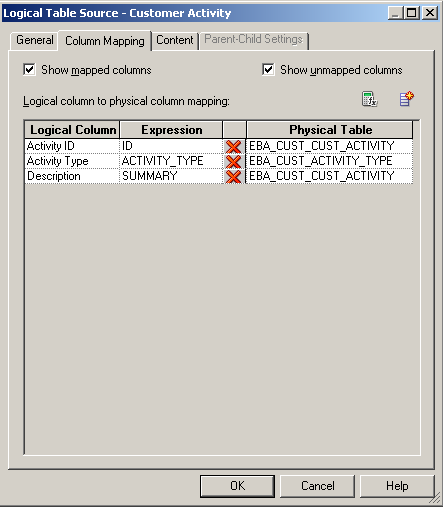
It’s also common to have interesting textual attributes existing in the same physical table that we are using as the source for our logical fact table. In our case, this is the EBA_CUST_CUST_ACTIVITY table, and the attribute that we are interested in is called SUMMARY. This attribute holds a description of the activity that has been performed. Although it’s debatable from a pure analytic perspective whether this attribute has value, it certainly does from an operational perspective, especially as an attribute when drilling down to the detail level of a report. When deciding what to do with this attribute, and how to make it available to the end user, we have a series of options. The first decision is a logical one: where do we put the logical column? We could put it in the logical fact table as a non-aggregating attribute, meaning an attribute that doesn’t participate in aggregate functions, but instead forms part of the GROUP BY statement. Although I think this is usually the wrong placement, it is the solution I see more than any others. It is difficult to educate an end user about aggregating and non-aggregating attributes in the same table, and some users will never fully get the distinction. The appropriate solution then is to place these interesting textual attributes, such as SUMMARY, in their own logical dimension table, even though the attributes exist in the “fact table”, so to speak. We can see the SUMMARY column, which has been placed in the logical dimension table Dim - Customer Activity and renamed to Description. I also add an additional table, EBA_CUST_ACTIVITY_TYPE to provide an Activity Type attribute to also use in the logical dimension table.

The reason we put this attribute in it’s own dimension is the importance of separating attributes from measures. Even though OBIEE supports the idea of delivering GROUP BY attributes directly in a logical fact table, that doesn’t mean we should use that feature. Placing the attribute in it’s own dimension also provides us the ability of reusing that dimension table as a conformed dimension table with other logical fact tables that may themselves have their own Description attribute that needs to be exposed, as Venkat describes in his post on modeling degenerate dimensions.

Once we have decided to place the Description attribute in the logical dimension table called Dim - Customer Activity, instead of placing it in Fact - Customer Activity, we now have a decision to make about how to construct the logical table source. The common approach I see is to construct two aliases of the source table, in this example, EBA_CUST_ACTIVITY: one to use as the dimension component of the table, and the other to use as the fact component. Even though I often see this approach, I still haven’t figured out why it is common. The preferred approach is to use the same physical source, either a single alias or a single physical table, as the source for both the dimension logical table source, and the fact logical table source.

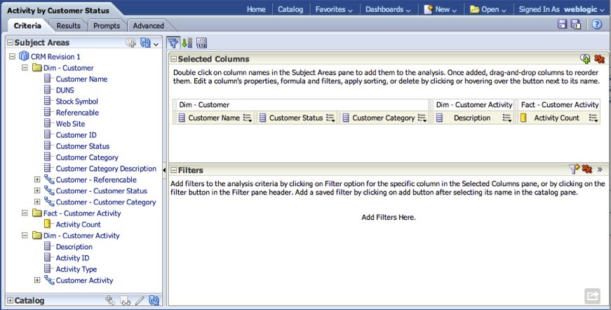
To compare these two approaches, I build the analysis using Dim - Customer, Dim - Customer Activity, and Fact - Customer Activity.

Using the 2 alias approach, we would get a self join to the EBA_CUST_ACTIVITY table: once as a dimension and once as a fact:

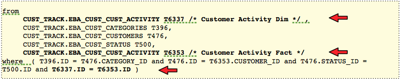
When using the same physical source for the fact table and the dimension, our report would display the same results, but we would get a single scan against the EBA_CUST_CUST_ACTIVITY table. The BI Server can make out the purpose of separating physical attributes in a logical manner and is capable of rendering the correct results with the fewest number of physical scans: