Experiments with Elastic’s Graph Tool

Robin Moffatt

Apr 29, 2016 • 15 min read

Elastic announced their Graph tool at ElastiCON 2016 (see presentation here). It’s part of the forthcoming X-Pack which bundles Graph along with other helper tools such as Shield and Marvel. Graph itself is two things; an extension of Elasticsearch’s capabilities, enabling the user to explore how items indexed in Elasticsearch are related, and a plugin for Kibana that acts as an optional front-end for this new functionality.

You can find a good introduction to Graph and the purpose and theory behind it in the documentation here. The installation of the components themselves is simple and documented here.

First Graph

To use Graph, you just point it at your existing data in Elasticsearch. The first data set I’m going to explore is one of the standard ones that everyone uses; Twitter. I'm streaming it in through Logstash (via Kafka for flexibility), but if you wanted you could ship it in via JDBC from any RDBMS, or from HDFS too.
See an important note at the end of this article about the slice of data within it, because it affects how the relationships visualised here should be viewed.

On launching Kibana’s Graph plugin (http://localhost:5601/app/graph) I choose the index (note that index patterns, e.g. when partitioning by date, are not supported yet), and the field in the data that I want to use as my vertices. A point to note here - “vertices” are usually called “nodes” in Graph terminology, but since Elasticsearch already uses “nodes” as part of its infrastructure topology terminology, they had to pick a different term.

In the search box, I can put my search term from which I’m interested to see the related ‘vertices’.

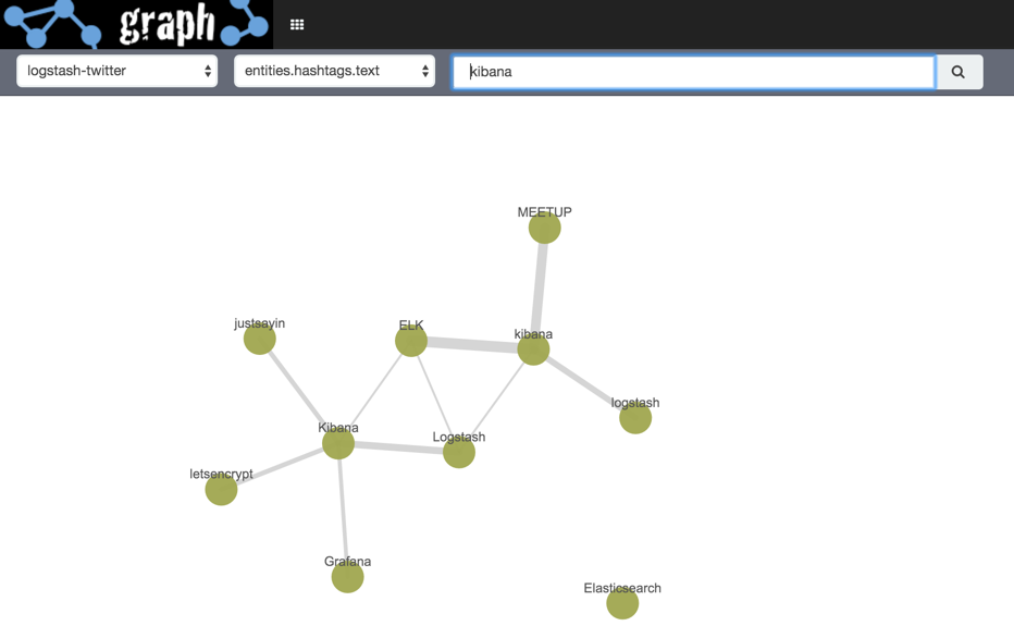
Sounds baffling? It is, kinda - right up until you run it (hit enter from the search box or click the magnifying glass search icon) and see what happens:

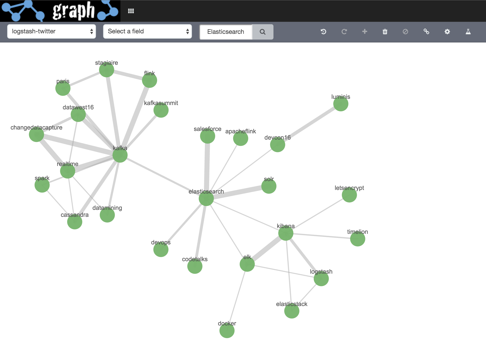
Here we’re seeing the hashtags used in tweets that mention Kibana. The “connections” (Elastic term) or “edges” (general Graph term) show which vertices (nodes) are related, and the width indicates the strength of that relationship (based on Elasticsearch's significant terms and scoring algorithm). For more details, see the "Behind the Scenes" section towards the end of this article.

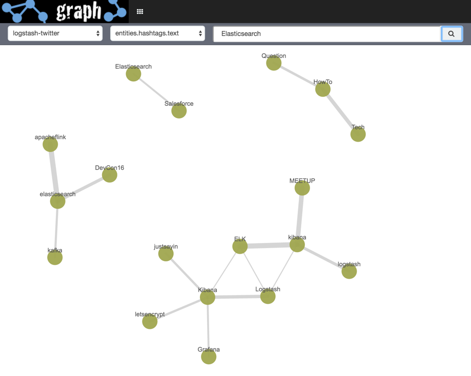
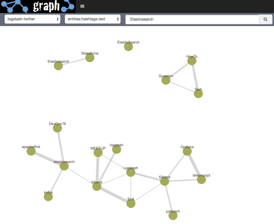
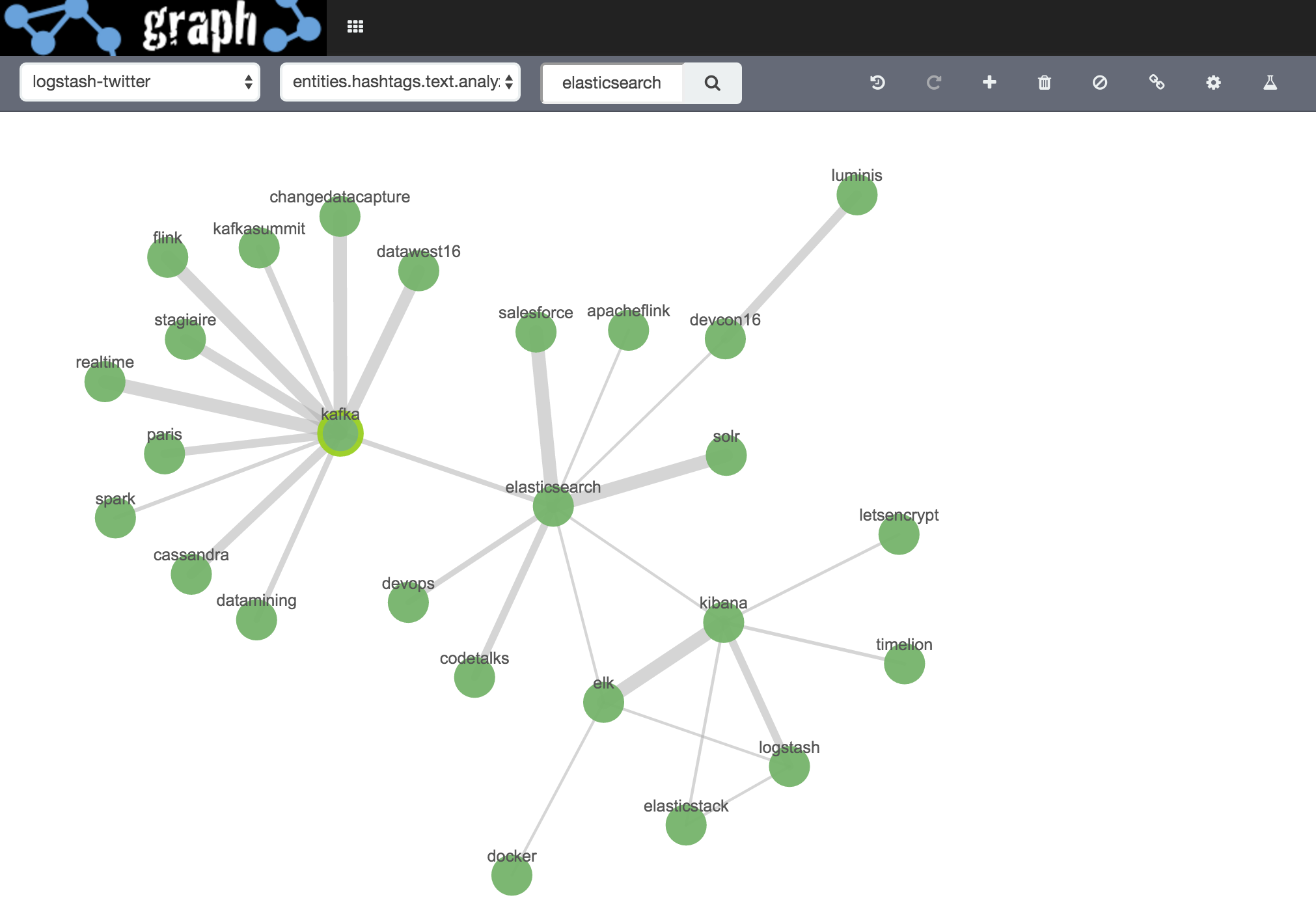
We can add in a second set of vertices by running a second search (“Elasticsearch”) - the results for these are, in effect, appended to the existing ones:

Add Links

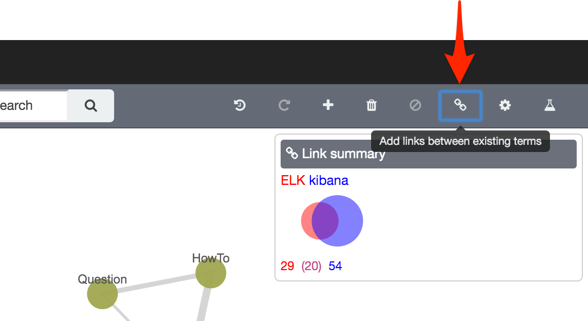
Since we’ve pulled back an additional set of vertices, it could be that there’s overlap between these and the first set (you’d kinda of expect it, Elasticsearch and Kibana being related). To visualise this, use the Add Links button

Note how the graph redraws itself with additional connections:

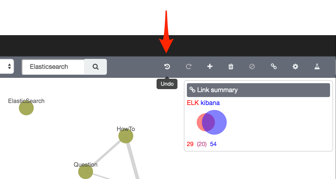
Blinked and you missed it? Use the Undo button to step back, and Redo button to re-apply.

Grouping Vertices

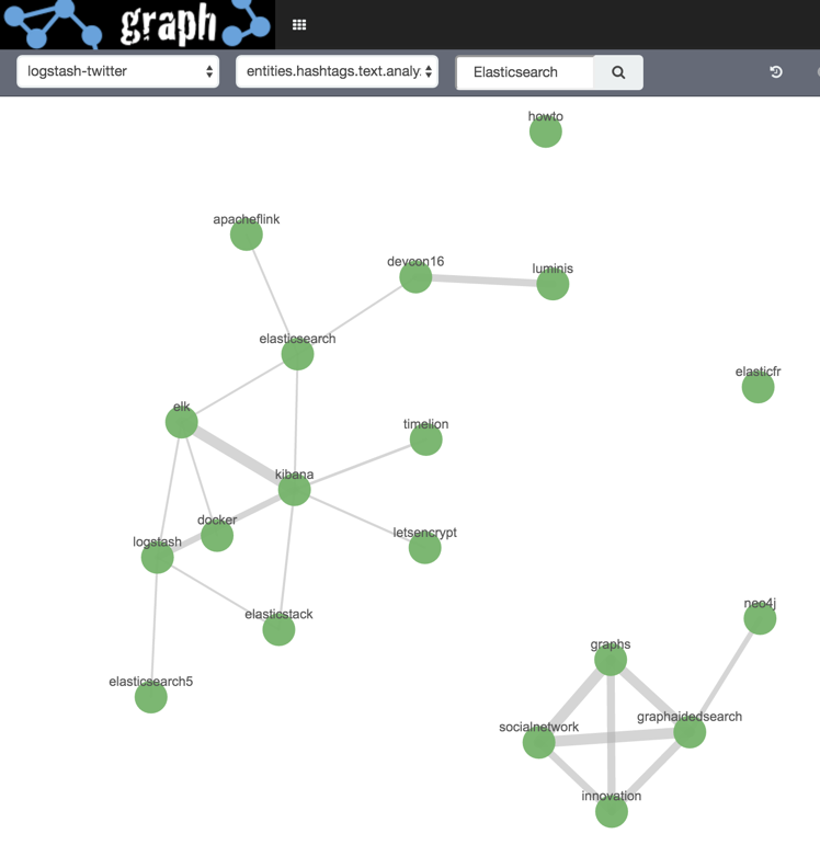
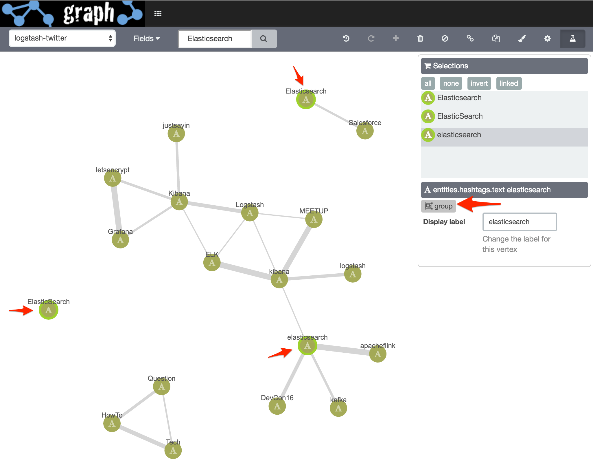
If you look closely at the graph you’ll see that Elasticsearch, ElasticSearch, and elasticsearch are all there as separate vertices. This is because I’m using a non-analyzed index field, so the strings are treated literally, case included. In this specific example, we’d probably re-run the graph using the analysed version of the field, which following the same two searches as above gives this:

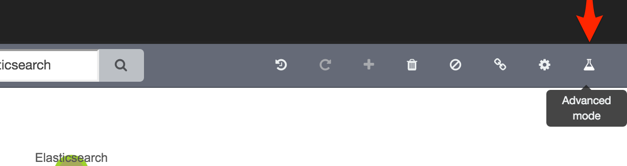
But, sticking with our non-analysed example, we can use it to demonstrate Graph’s ability to group multiple terms together into a single vertex. Switch to Advanced Mode:

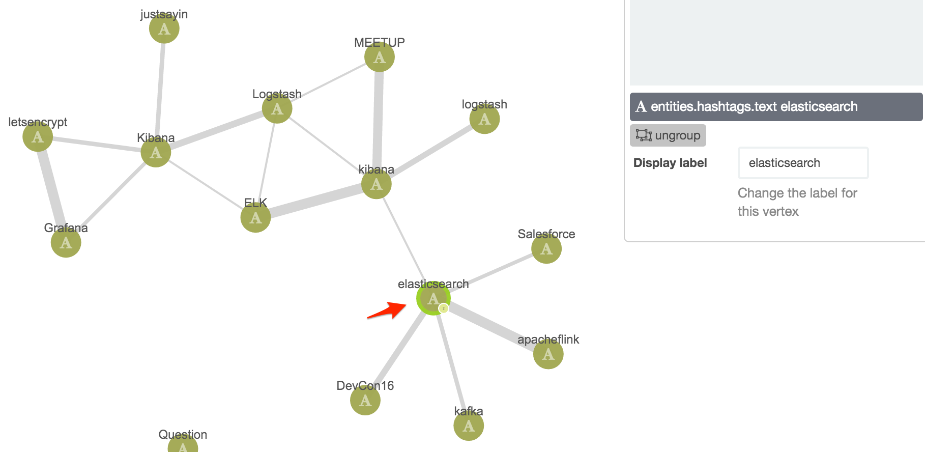
and then select the three vertices and click the group option

Now all three, and their connections, are as one:

Whilst the above analysed/non-analysed difference gave me excuse to show the group function (can you tell I’ve done many-a-failed-live-demo? ;-) ), I’m now going to switch over to a graph built on the analysed version of the hashtag field, as we saw briefly above:

Tidying up the Graph - Delete and Blacklist

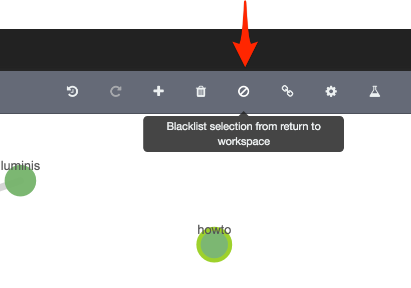
There’s a few straglers on the Graph that are making it less easy to comprehend. We can temporarily remove them, or even blacklist them from appearing again in this session:

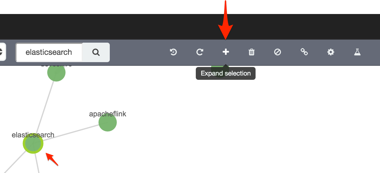
Expand Selection

One of the points of Graph analysis is visualising the relationships in your data in a way that standard relational methods may not lend themselves to so easily. We can now start to explore this further, by digging into the Graph that we’ve got so far. This process, along with the add links seen above, is often called "spidering". By selecting the elasticsearch node and clicking on Expand selection we can see additional (by default, five) vertices related to this one:

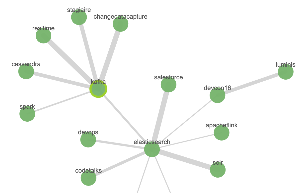
So we see that kafka is related to Elasticsearch (in the view of the twitterati, at least), and let’s expand that Kafka vertex too:

By clicking the Expand selection button again for the same vertex we get further results added:

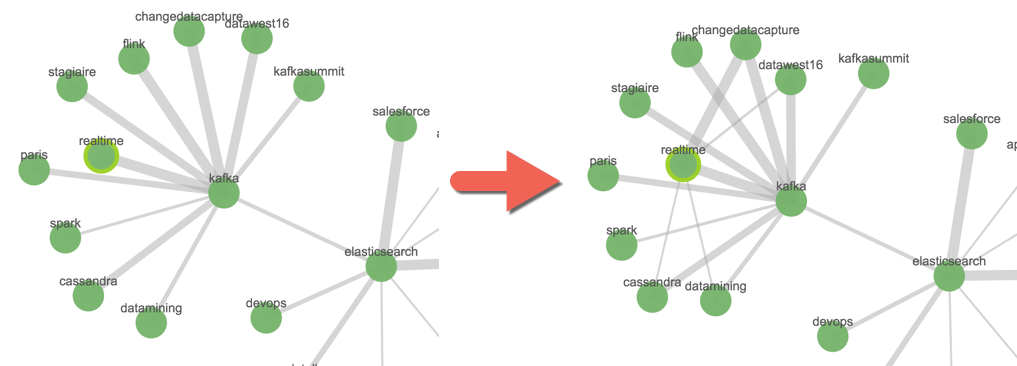
We can select one node (e.g. realtime) an using the Add Link see additional relationships:

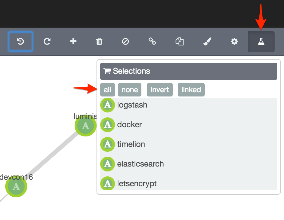
But, there are many nodes, and we want to see any relationships. So, switch to Advanced Mode, select All…

…add Add Link again:

Knob Twiddling

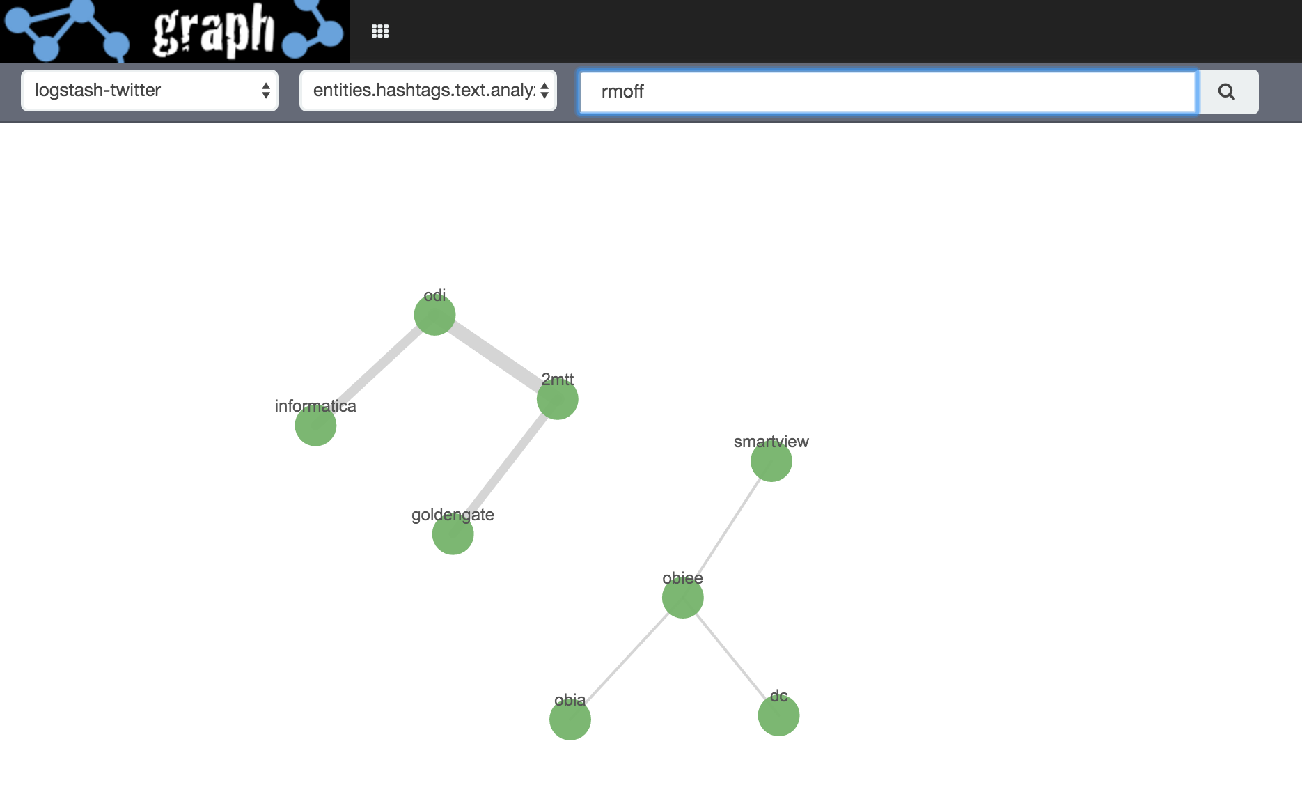
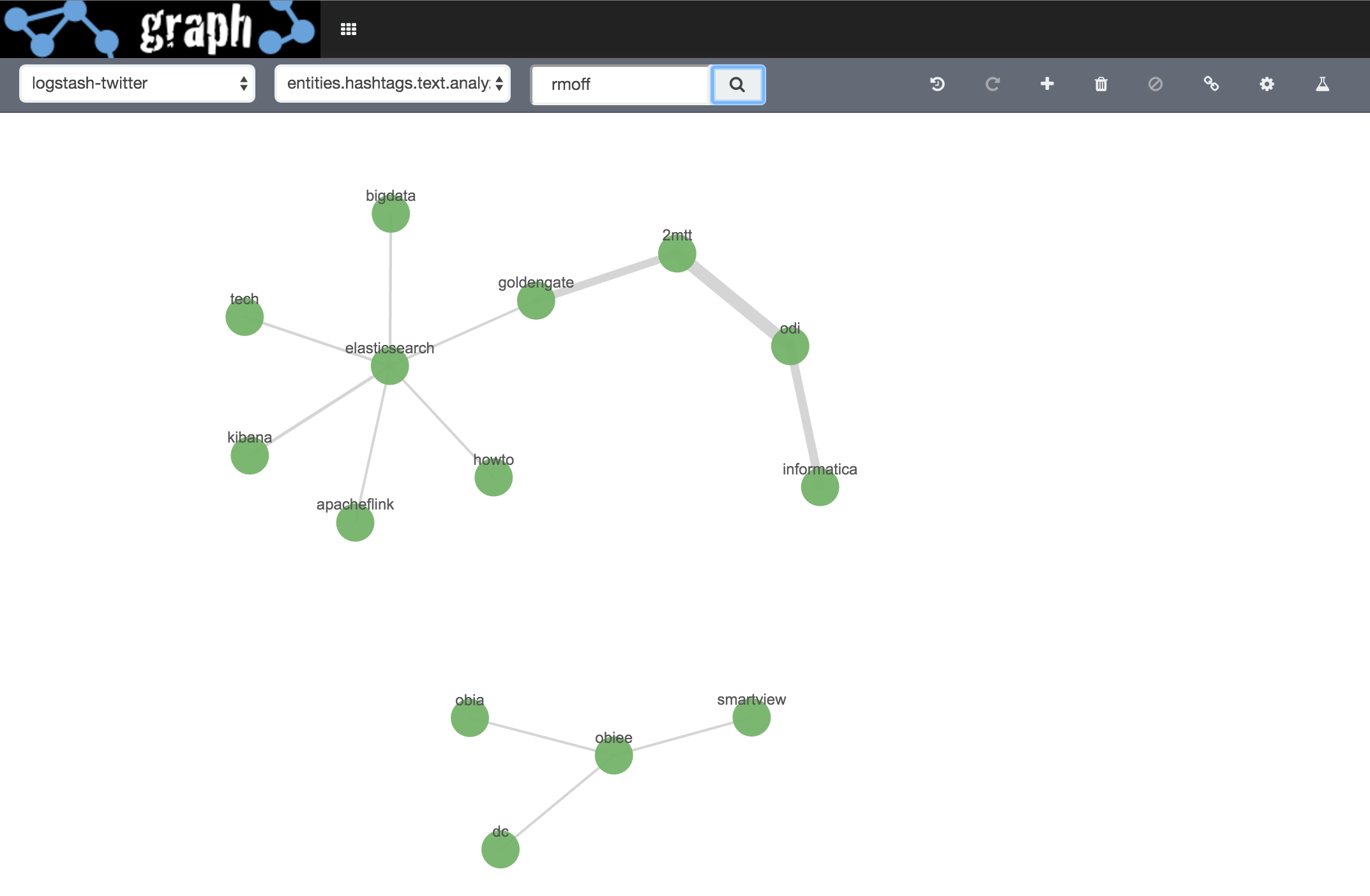
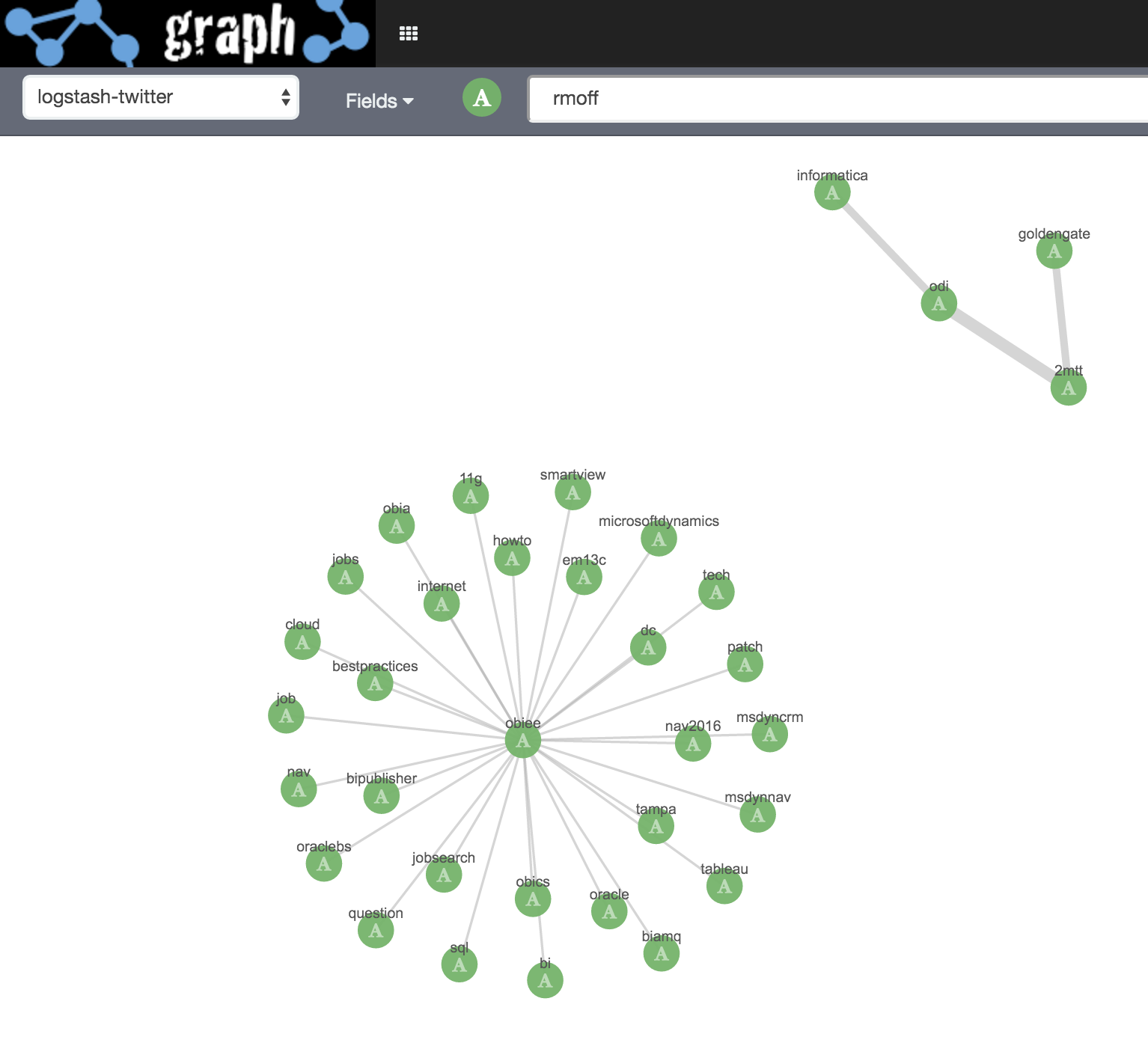
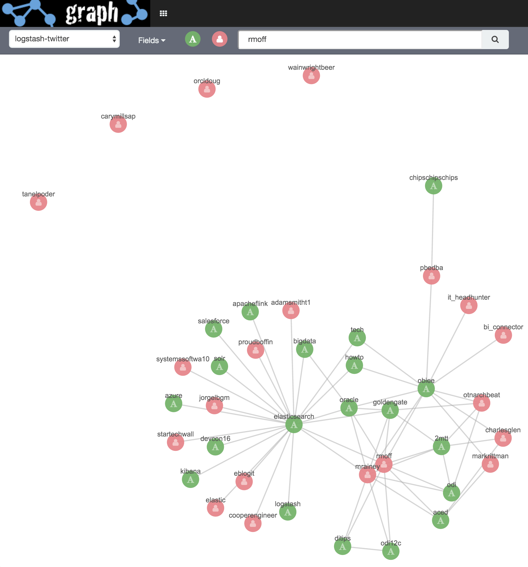
Let’s start with a blank canvas, in basic mode, showing hashtags related to … me (@rmoff)!

But, surely I do more than talk about OBIEE and ODI? Like, Elasticsearch? Let’s relax the Graph selection criteria, under Settings:

and run the search again (on top of the existing results):

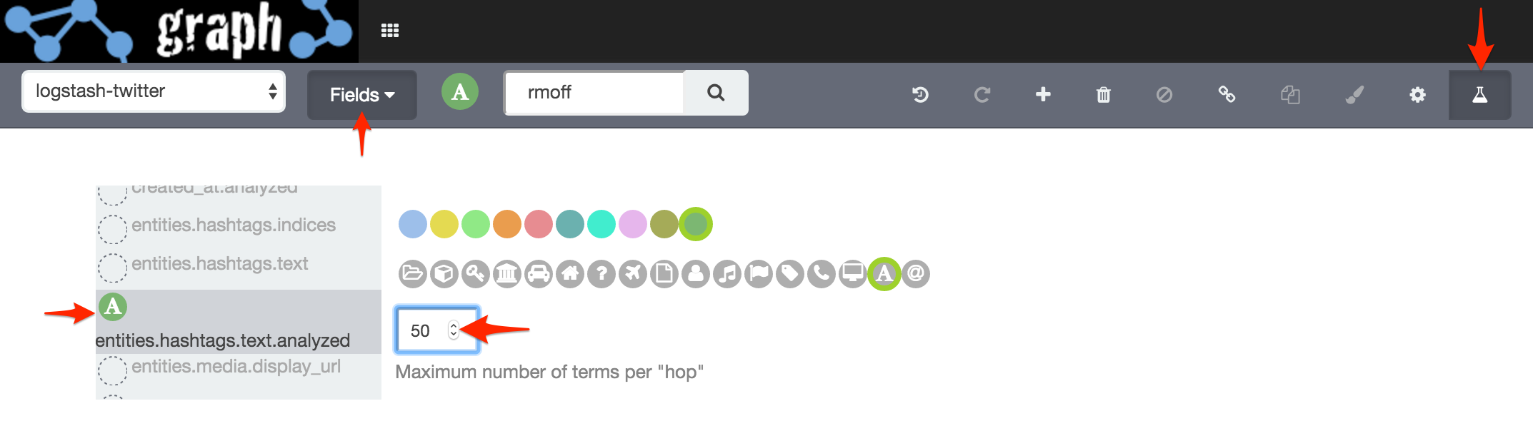
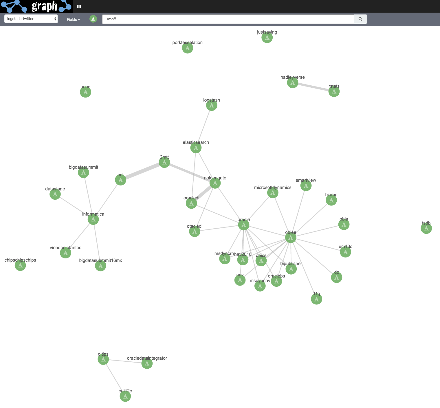
There’s more results … but I know how much I tweet and it feels like I’m only seeing a part of the picture. By switching over to Advanced Mode, we can refine how many results each field returns:

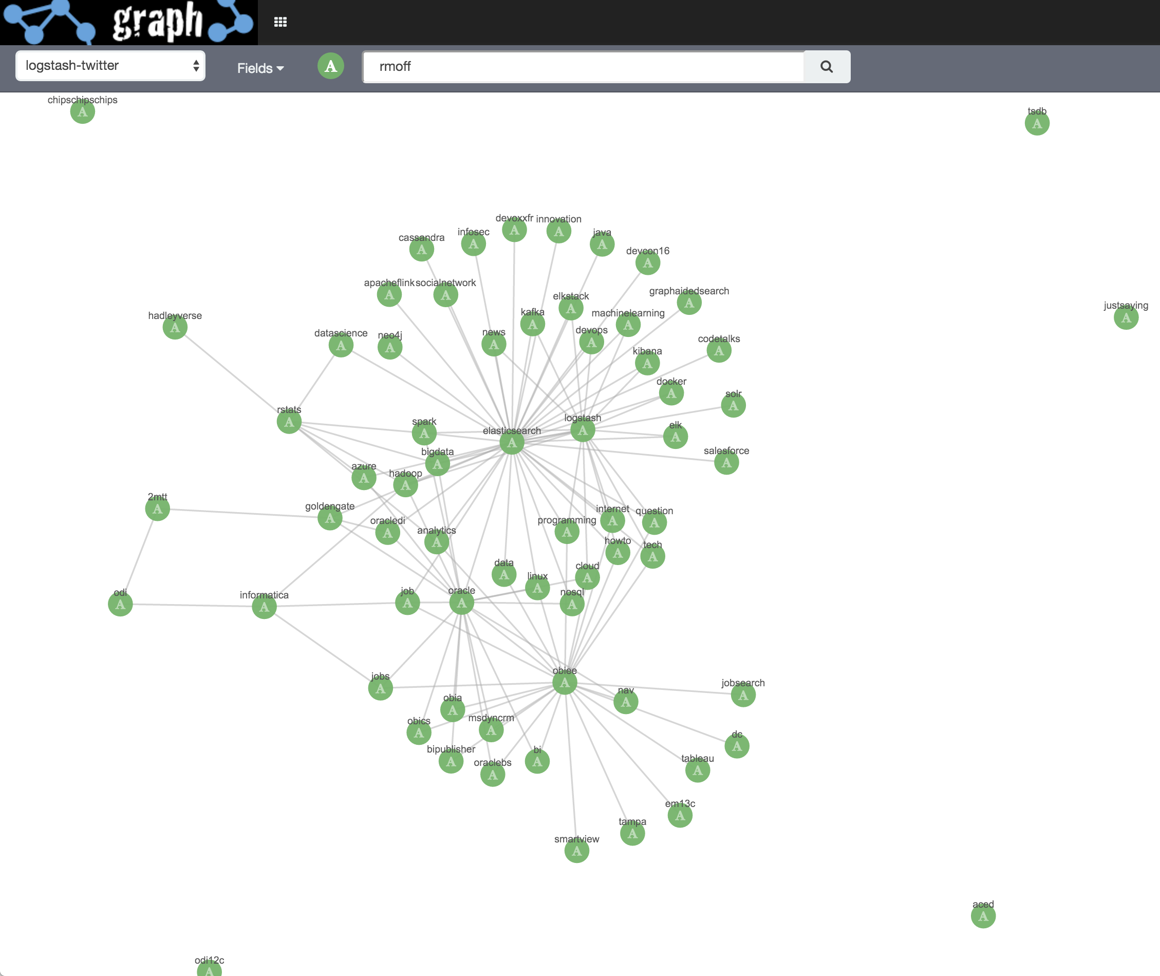
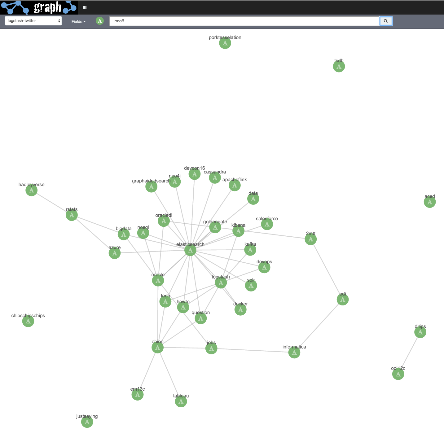
I reset the workspace (undo to blank, or just reload), and run the search again, this time with a greater number of hashtag field values shown, and with the same relaxed search settings as shown above:

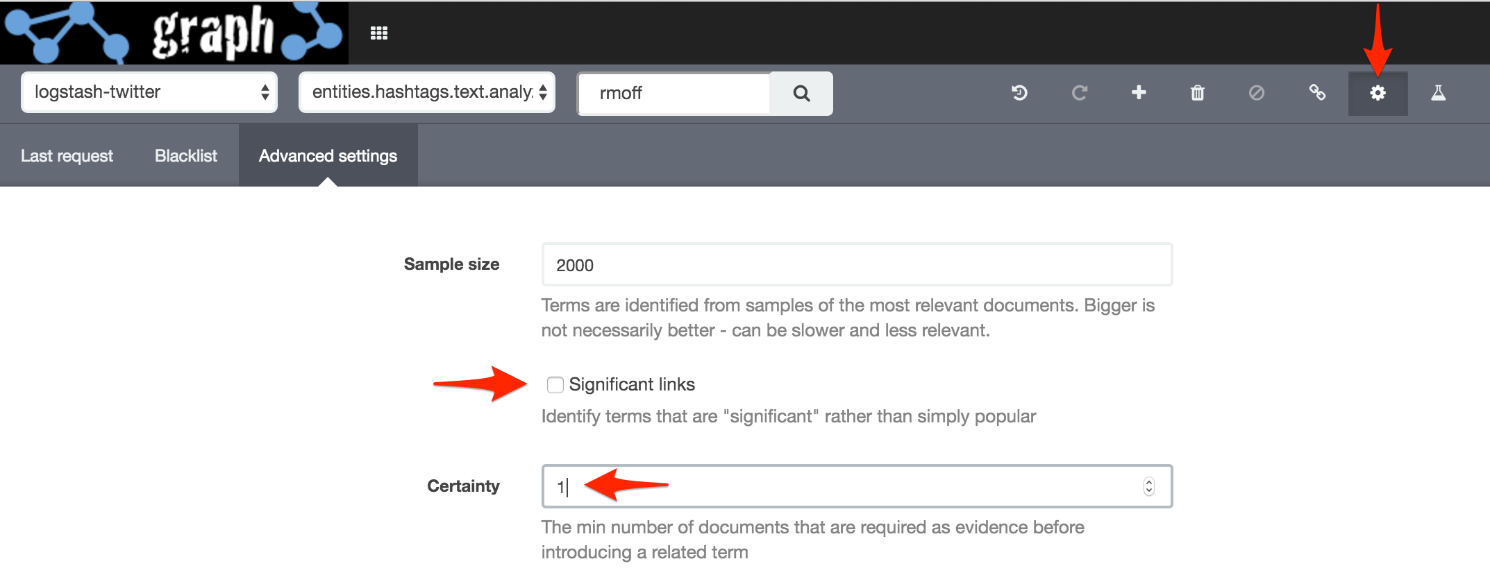
At this point I’m into “fiddling” territory, twiddling with the ‘Number of terms’, ‘Significant’ and ‘Certainty’ knobs to see how the results vary. You can read more about the algorithm behind the Significance setting here, and more about the Graph API here. The certainty setting is simply "The min number of documents that are required as evidence before introducing a related term", so by lowering it we see more links, but potentially with more "noise" too, of terms that aren't really related.

An important point to note here is the dataset that I’m using is already biased because of the terms I’m including in my twitter feed search, therefore I’d expect to see this skew in the results below. See the section at the end of this article for more details of the dataset.

50 terms, significant unticked, certainty 1 (as above)
50 terms, significant ticked, certainty 1
50 terms, significant ticked, certainty 3
20 terms, significant ticked, certainty 1
20 terms, significant unticked, certainty 1

Based on the above, "Significant" seems to reduce the number of relationships discovered, but increase the level of weight shown in those that are there.

Adding Additional Vertex Fields

So we’ve seen a basic overview of how to generate Graphs, expand selections, and add relationships to those additional selections. Let’s look now at how multiple fields can be added to a Graph.

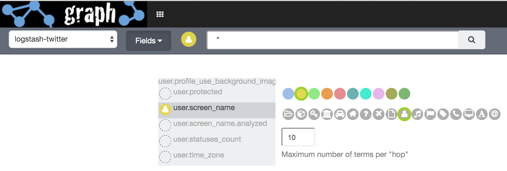
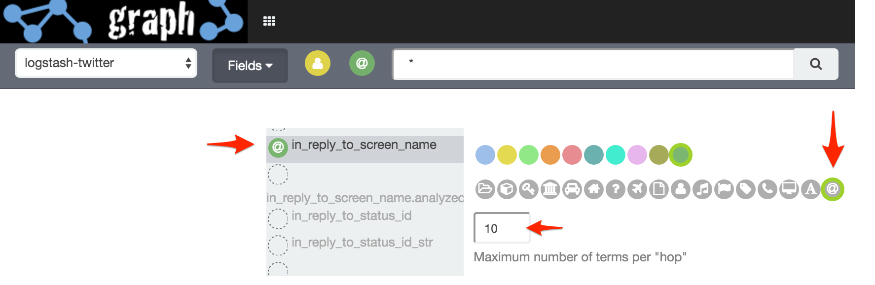
Starting with a blank workspace, I switched to Advanced Mode and added two fields from my twitter data:

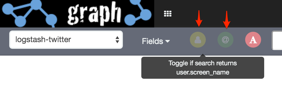
user.screen_name
in_reply_to_screen_name

Note that you can customise the colour and icon of different fields.

Under Options I’ve left Significant Links enabled, and set Certainty to 1.

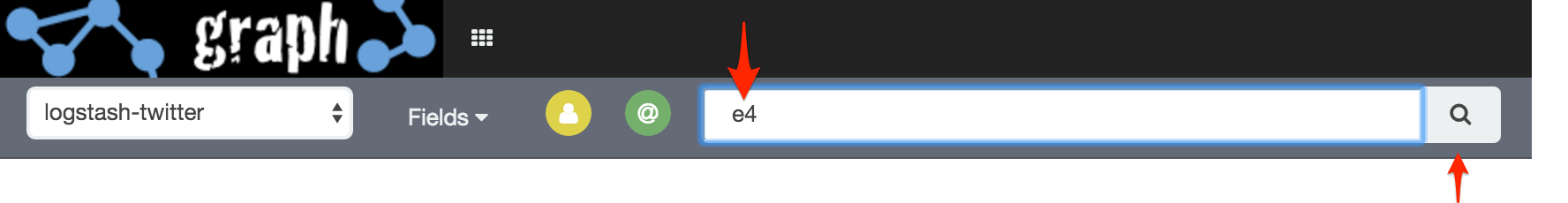
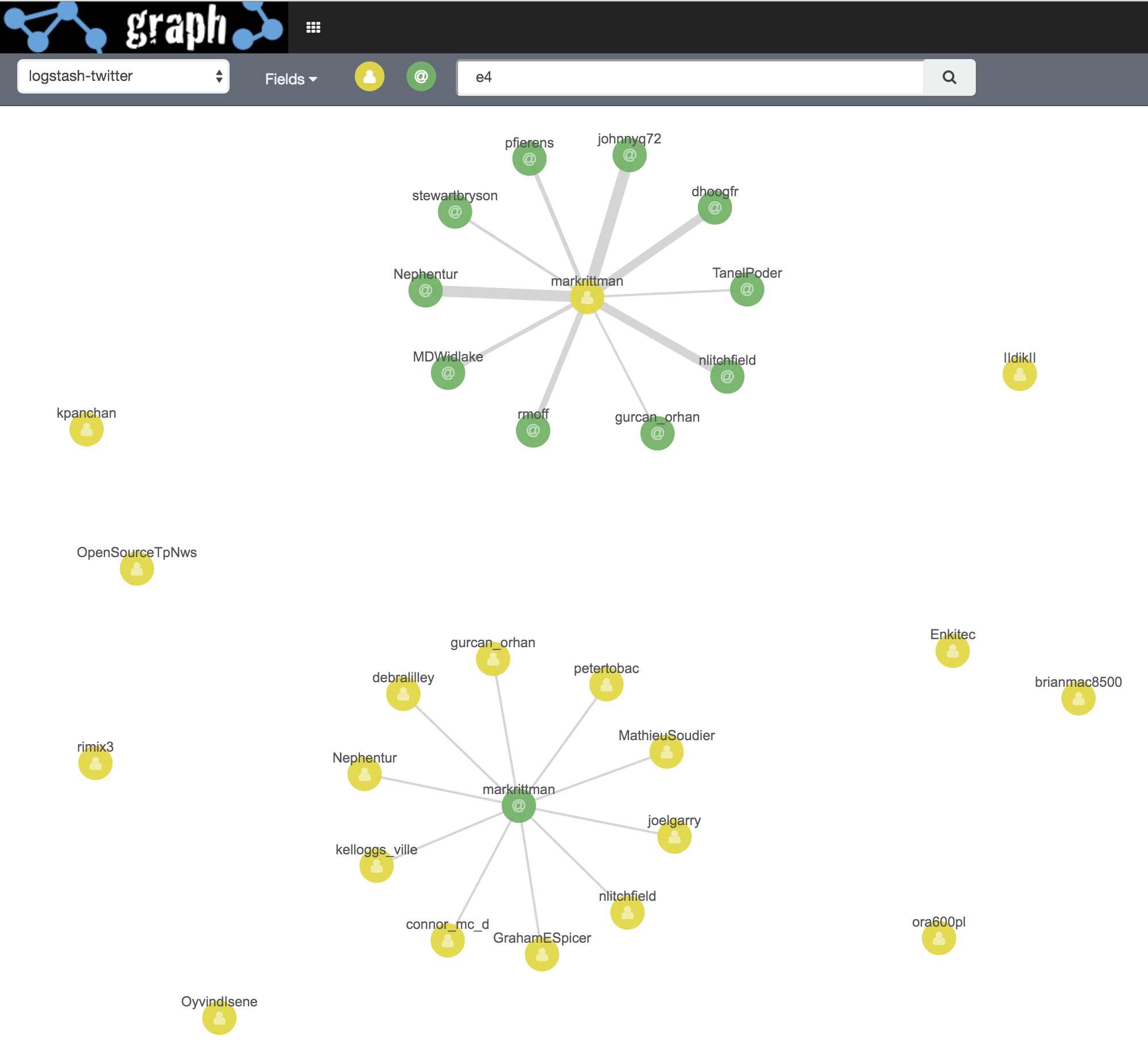
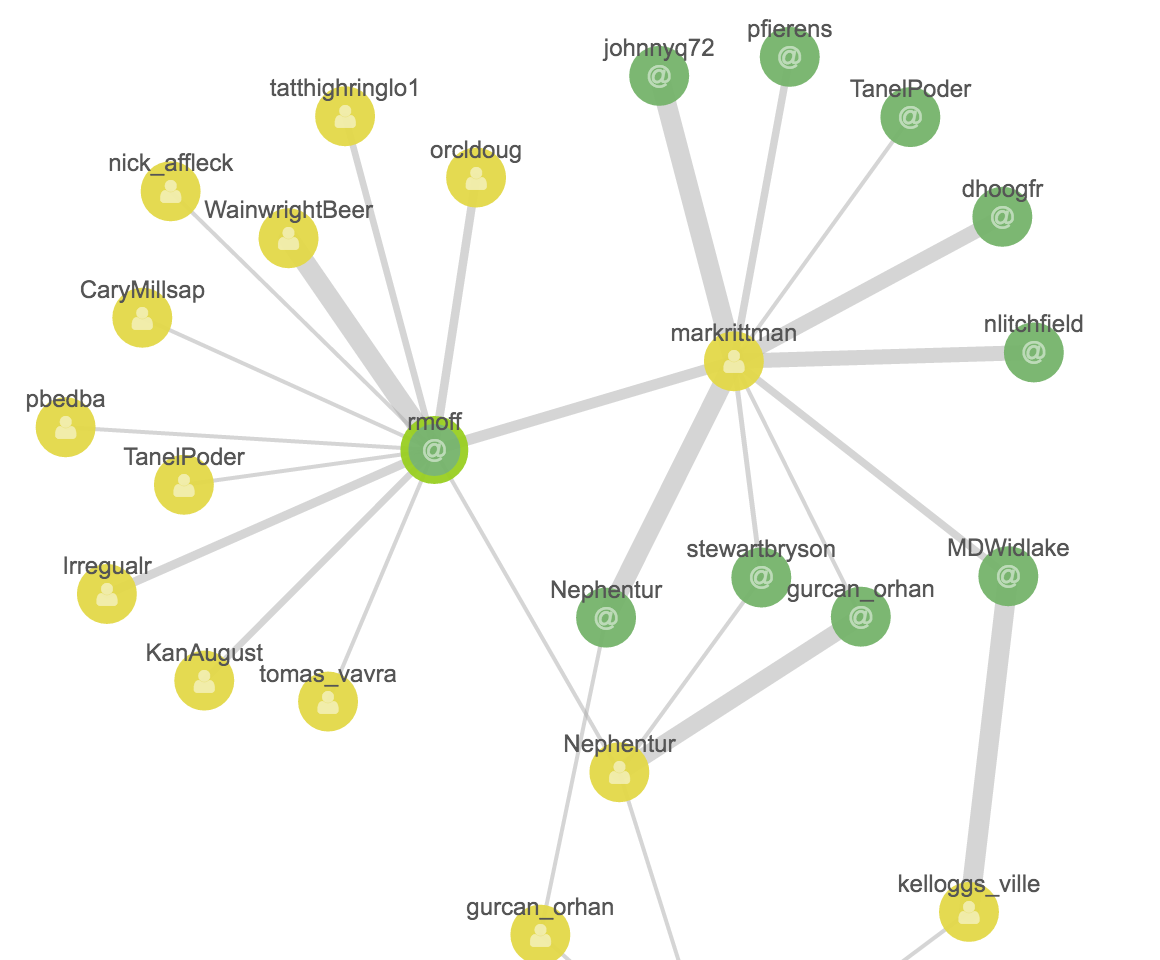
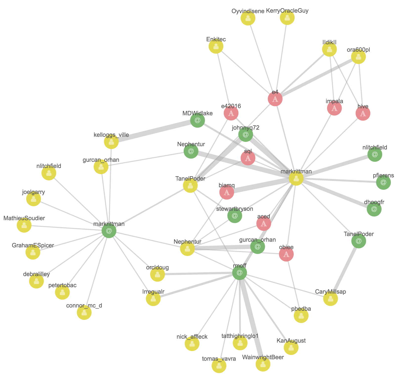
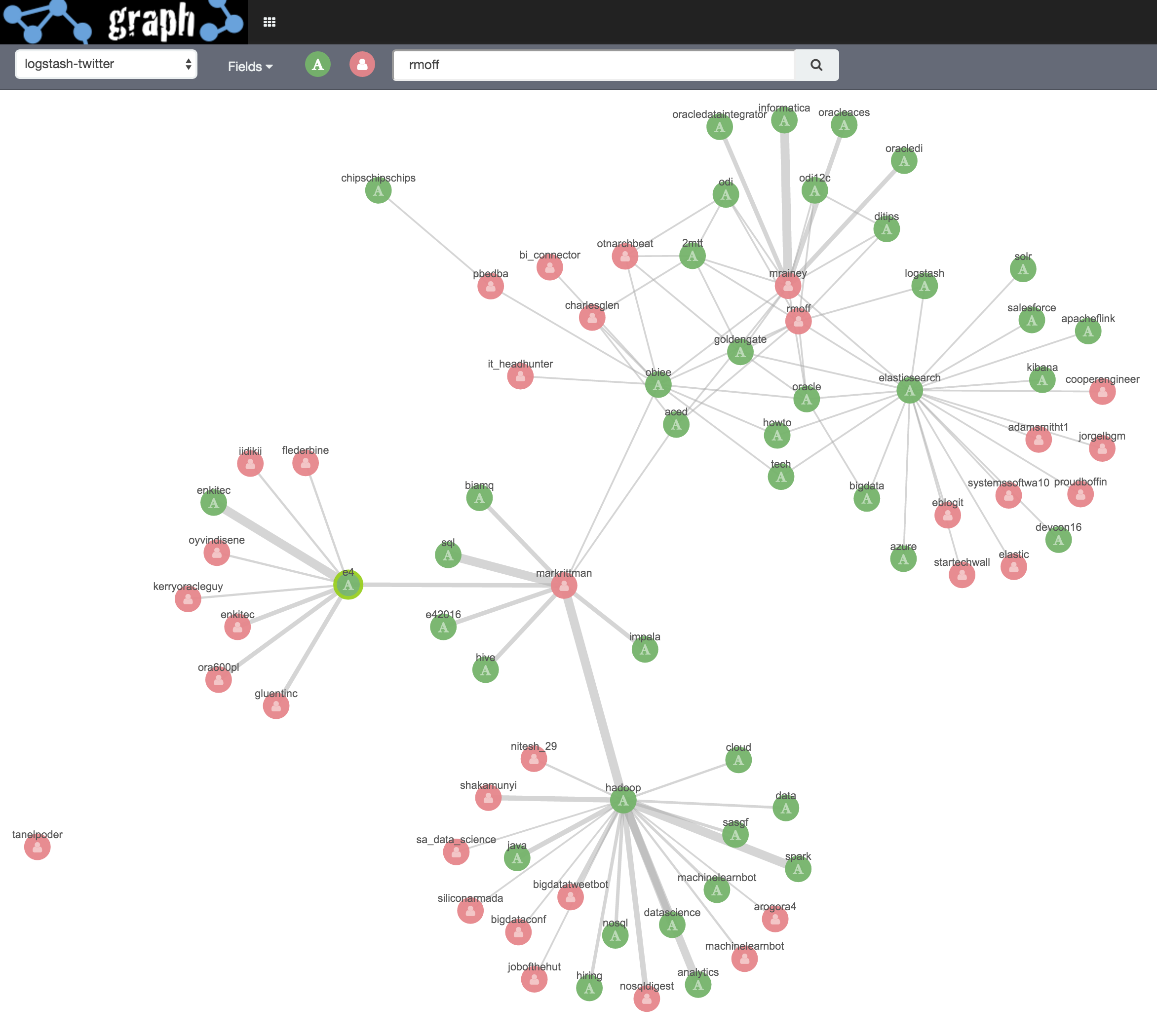
Let’s see who’s been interacting about the recent E4 summit:

Whilst it looks like Mark Rittman is the centre of everything, this is actually highlighting a skew in the source dataset - which includes everything Mark tweets but not all tweets about E4. See the section at the end of this article for more details of the dataset.

The lower cluster is Mark as the addressee of tweets (i.e. he is the in_reply_to_screen_name), whilst the upper cluster is tweets that Mark has sent addressing others (i.e. he is the user.screen_name).

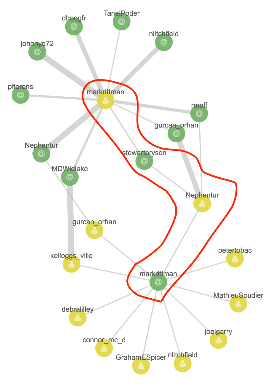
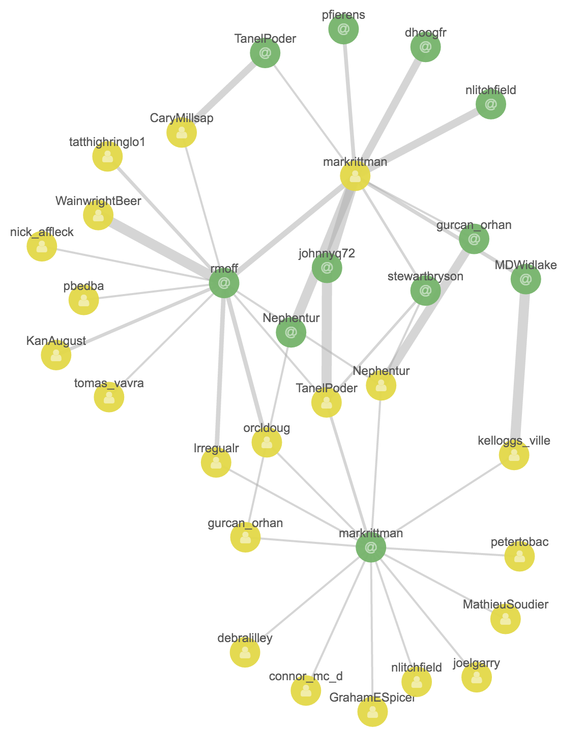
If we click on Add Links a couple of times we can see that there’s other connections here - for example, Mark replies to Stewart (@stewartbryson), who Christian Berg (@Nephentur) talks to, who in turn talks to Mark.

This being twitter and the age of narcissism, I’ll click on my vertex and click Expand Selection to see the people who in turn talk to me:

And by using Add Link see how they relate to those already shown in the Graph:

Viewing Associated Records

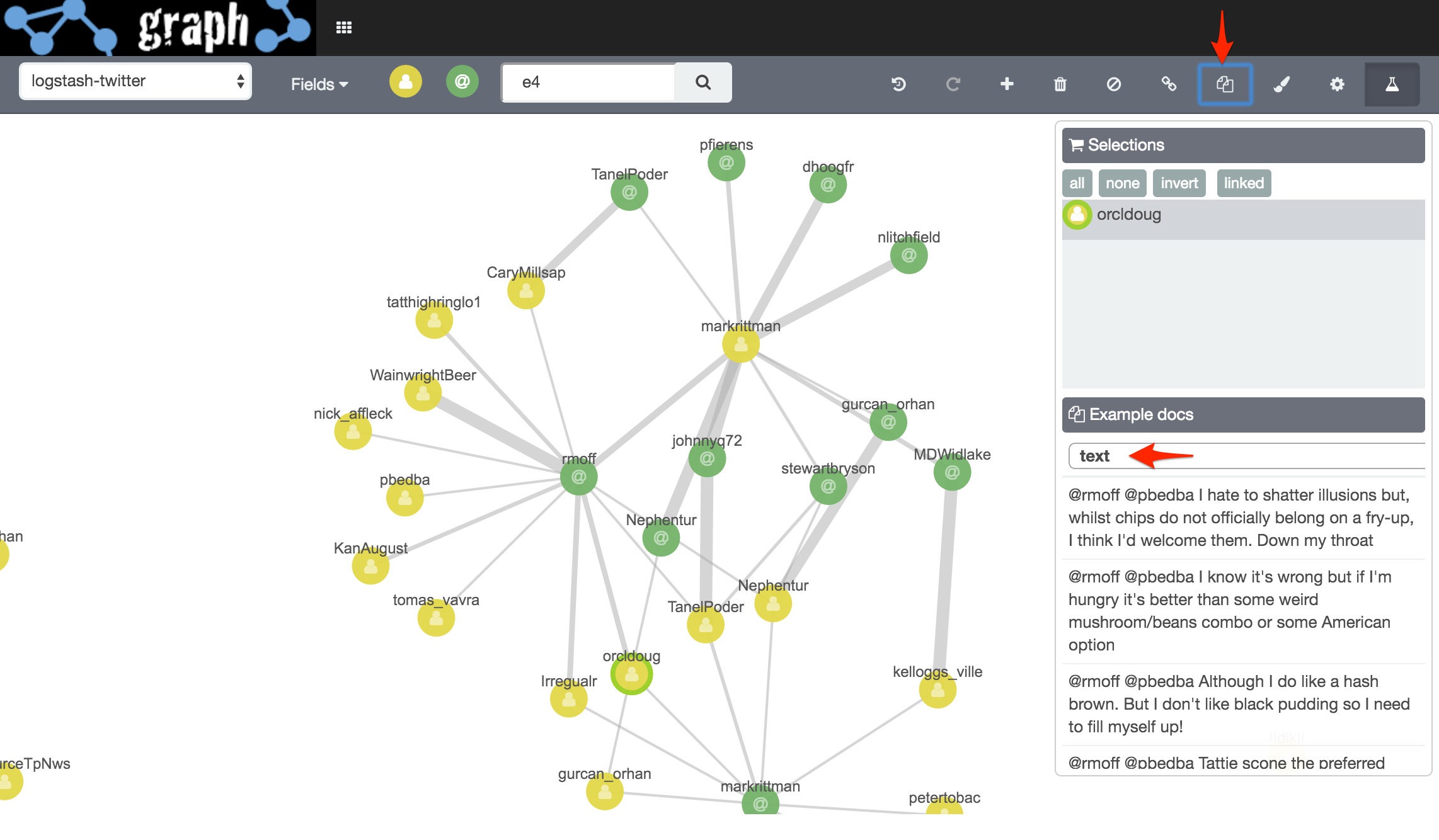
Within Graph there’s the option to view the data associated with one or more vertices. We do this by selecting a vertex and clicking on View Example Docs (in Elasticsearch parlance, a document is akin to a ‘row’ as traditional RDBMS folk would know it). From here select the field - for twitter the text field has the contents of the tweet:

Adding Even more Vertex Fields

So, we’ve got a bit of a picture of who talks to whom, but can we see what they’re talking about? We could use the text field shown above to see the contents of tweets but that’s down in the weeds of individual tweets - we want to step back a notch and get a summarised view.

First I add in the hashtag field:

And then deselect the two username fields. This is so that I can expand existing vertices, and instead of showing related hashtags and users, instead I only expand it to show hashtags - and not additional users.

Now I select Mark as the orinator of a tweet, and Expand Selection followed by Add Links on all vertices until I get this:

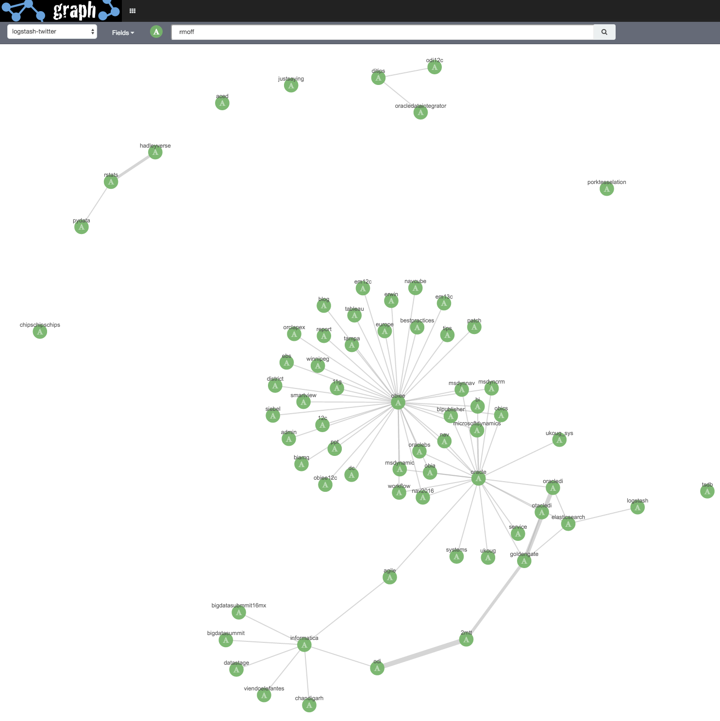
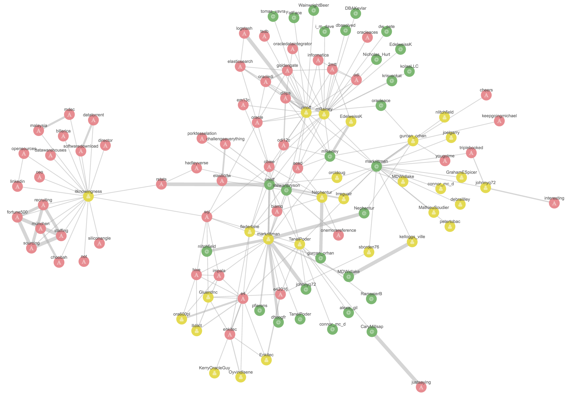
The number of values selected is key in getting a representative Graph. Above I used a value of 10. Compare that to instead running the same process but with 50. Under Options I’ve left Significant Links enabled, and set Certainty to 1:

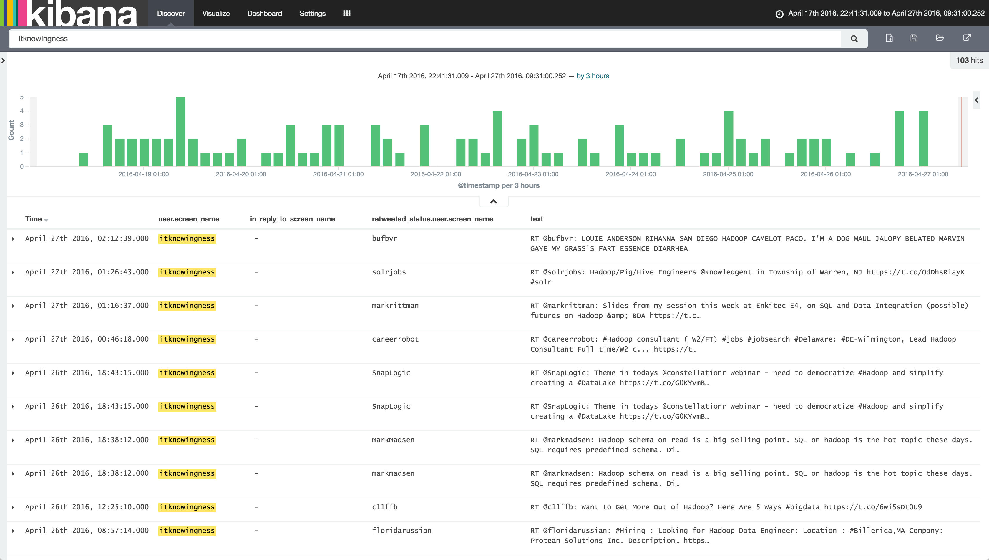
One interesting point we can see from this is that the user “itknowingness” in the cluster on the left seems to use all the hashtags, but doesn’t interact with anyone - from the Graph it’s easy to see, and a great example of where Graph gives you the answer to a question you didn’t necessarily know that you had, and which to get the answer out through a traditional RDBMS query would need a very specific query to do so. Looking at the source data via Kibana’s Discover panel shows that it is indeed a bot auto-retweeting anything and everything:

Building a Graph from Scratch

Now that we’ve seen all the salient functions, let’s start with a blank canvas, and see where we get.
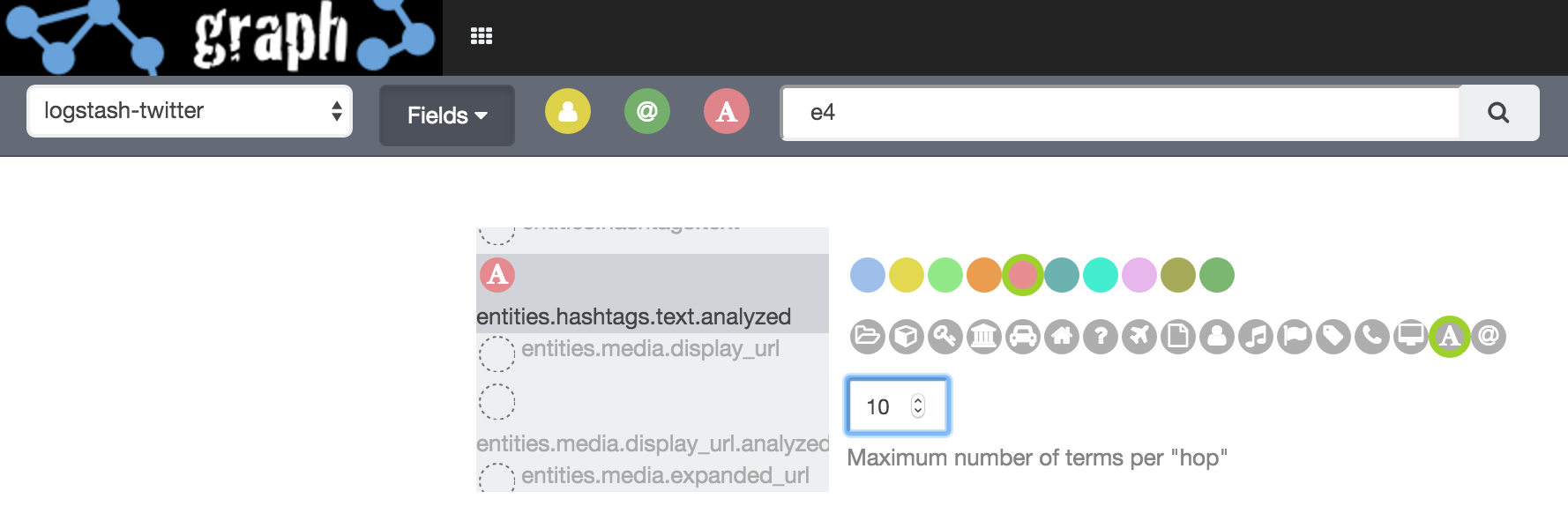
The setttings I’m using are:

Significant Links unticked
Certainty = 1
Field entities.hashtags.text.analyzed max terms = 10
Field user.screen_name max terms = 10
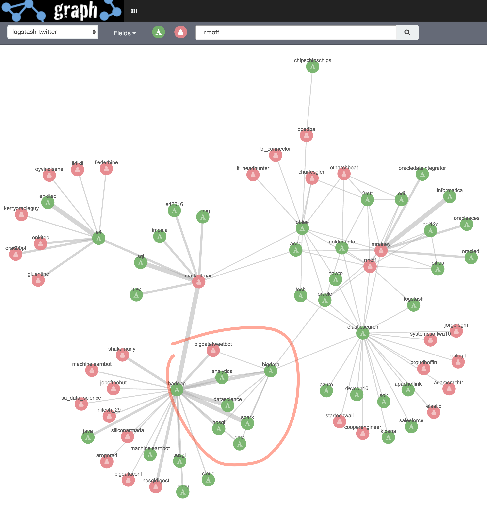
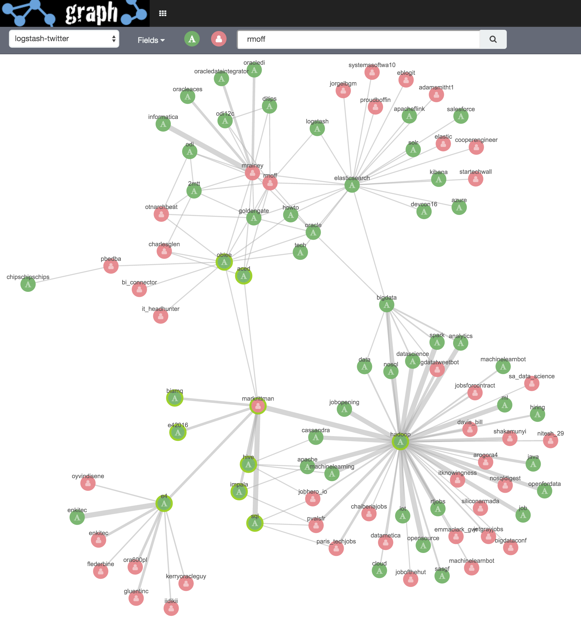
Initial search term rmoff

Then I click on markrittman and Expand Selection, the same for mrainey, and also for the two hashtags e4 and hadoop:

Within the clusters, let’s see what links exist. With no vertices select I click on Add Links (which seems to be the same as selecting all vertices and doing the same). With each click additional links are added, all related to the hadoop/bigdata area:

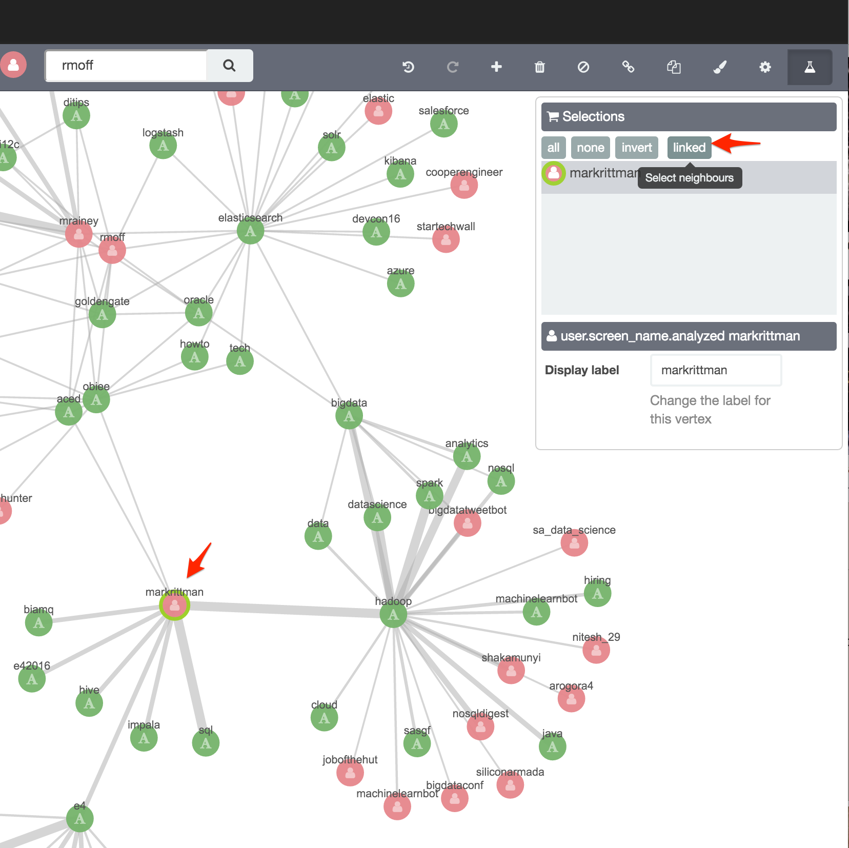
I’m interested now in the E4 region of the Graph, and the vertices related to Mark Rittman. Clicking on his vertex and clicking “Select Neighbours” does exactly that:

Now I’m more interested in digging into the terms (hashtags) that are related that people, so I deselect the user.screen_name field, and then Expand Selection and Add Links again.

Note the width of the connections - a strong relationship between Mark Rittman, “Hadoop” and “SQL”, which is presumably from the tweets around the presentation he did recently on the subject of… SQL on Hadoop. Other terms, including Hive and Impala, are also related, as you’d expect.

Graphing Tweet Text Contents

By making sure that the tweet text is available as an analysed field we can produce a Graph based on the ‘tokens’ within the tweet, rather than the literal 140 characters. Whilst hashtags are there deliberately to help with the classification and grouping of tweets (so that other people can follow conversations on the same subject) there are two reasons why you’d want to look at the tweet text too:

Not everyone uses hashtags
Not all relationships are as boolean as a hashtag or not - maybe a general discussion in an area re-uses the same words which overall forms a relationship between the terms.

Here I’m going back to the default settings:

Significant Links ticked
Certainty = 3

And returning two fields - hashtag and tweet text

Field entities.hashtags.text.analyzed max terms = 20
Field text.analyzed max terms = 50
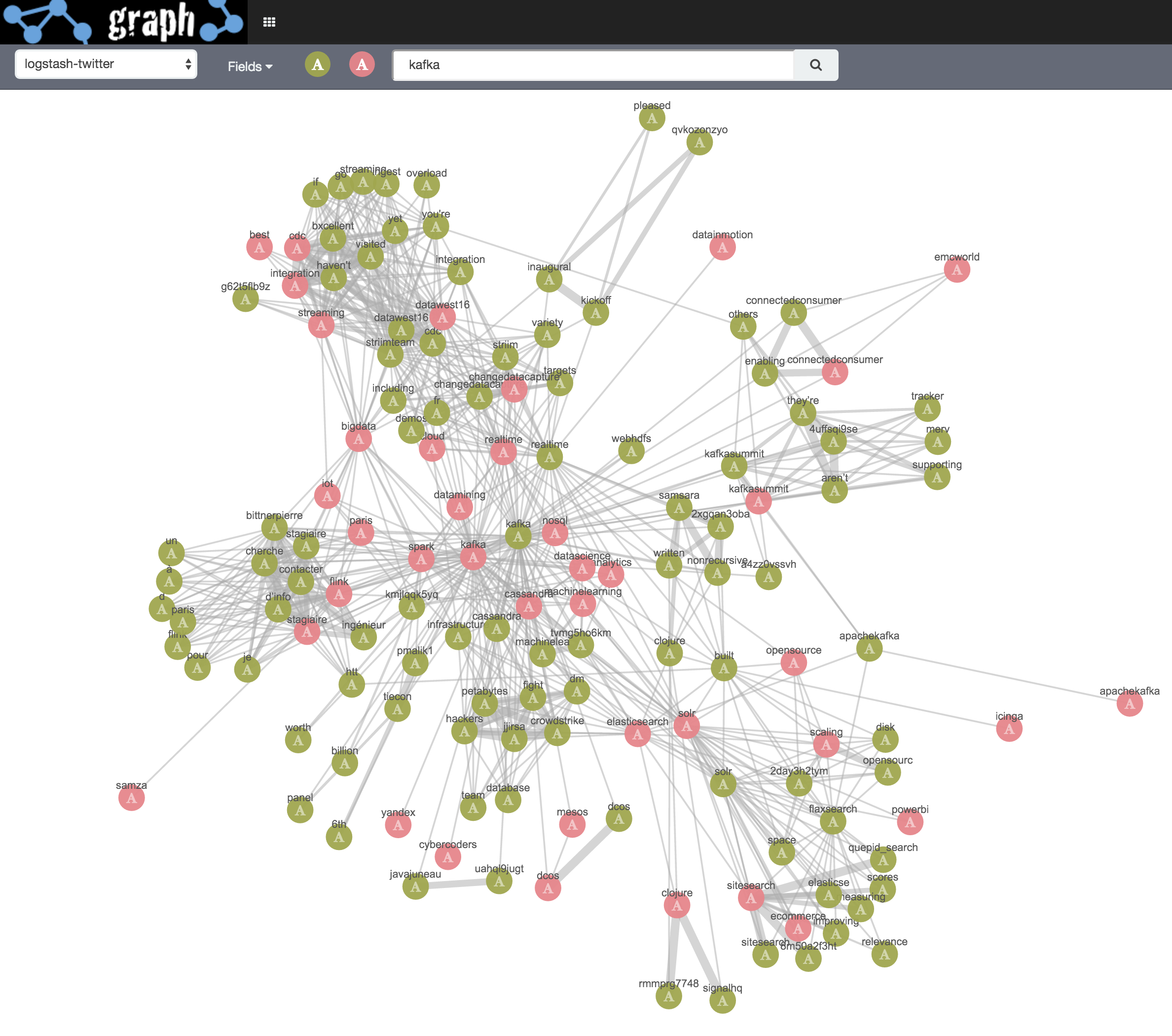
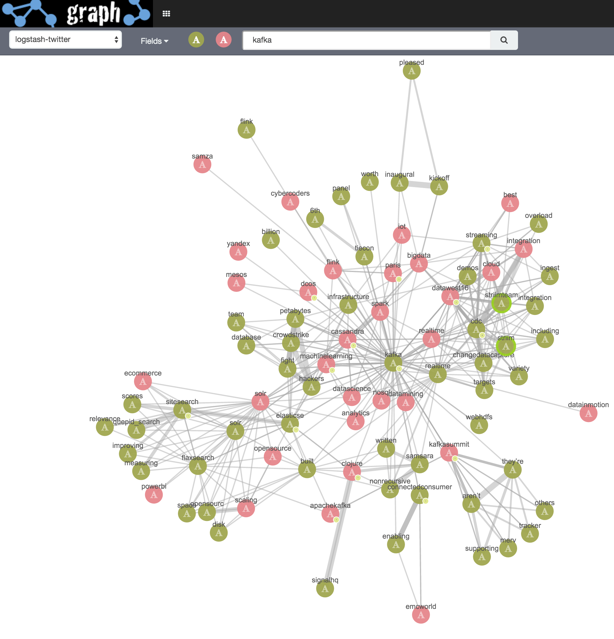
Initial search term kafka

I then tidy it up a bit :

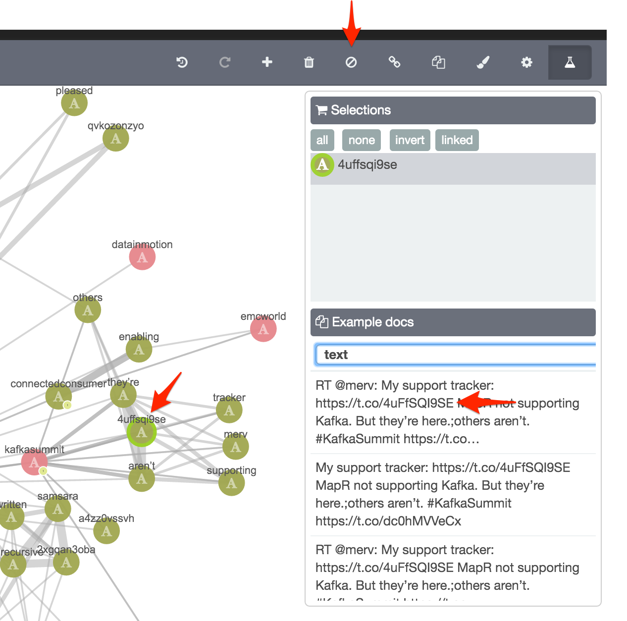
Joining the same/near-same text and hashtags, such as “kafkasummit” hashtag and the same text. If you think about the contents of a tweet, hashtags are part of the text, therefore, there’s going to be a lot of this duplication.
Blacklisted text terms that are URL snippets. Here I’m using the Example Docs function to check the context of the term in the whole text field
I also blacklisted common words (“the”, “of”, etc), and foreign ones (how British…).

Behind the Scenes

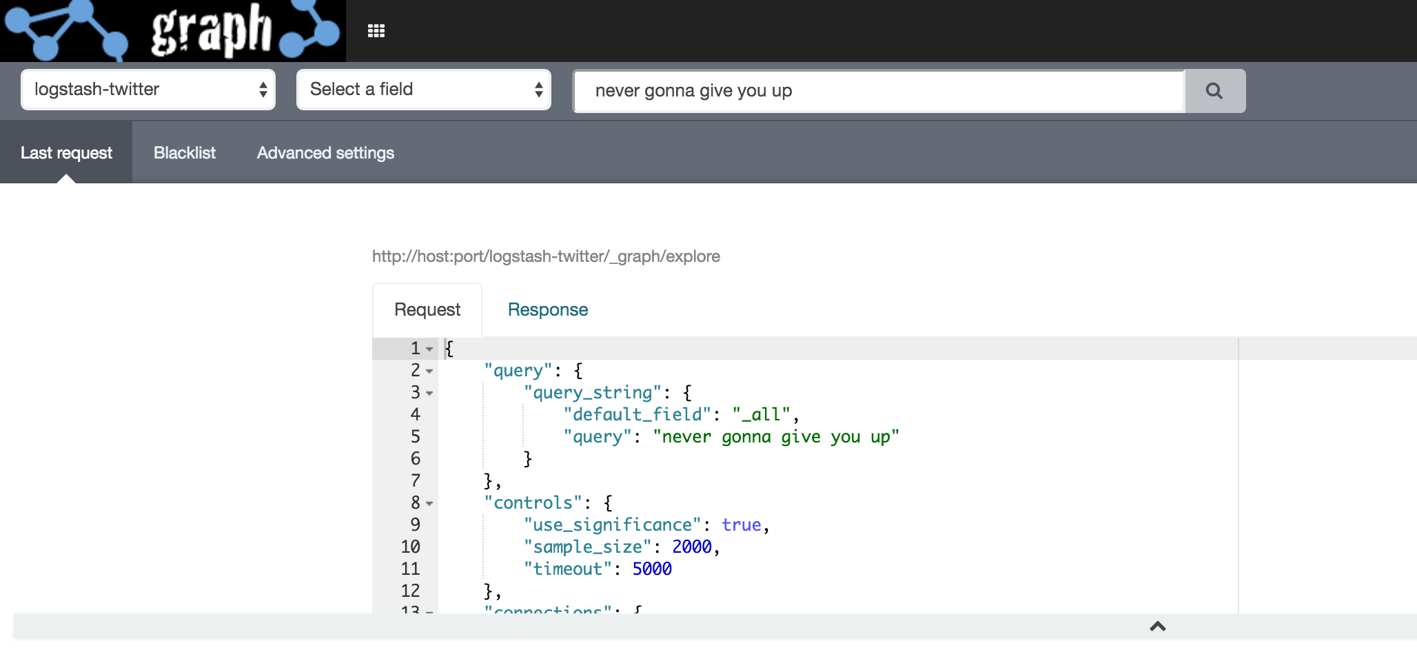
The Kibana Graph plugin is just a front-end for the Graph extension in Elasticsearch. It’s useful (and fun!) for exploring data, but in practice you’d be making direct REST API calls into Elasticsearch to retrieve a list of vertices and connections and relative weights for use in your application. You can see details of this from the Settings page and Last Request option

Looking at an example (the one used in the first example on this article), the request is pretty simple:

{
    "query": {
        "query_string": {
            "default_field": "_all",
            "query": "kibana"
        }
    },
    "controls": {
        "use_significance": true,
        "sample_size": 2000,
        "timeout": 5000
    },
    "connections": {
        "vertices": [
            {
                "field": "entities.hashtags.text.analyzed",
                "size": 5,
                "min_doc_count": 3
            }
        ]
    },
    "vertices": [
        {
            "field": "entities.hashtags.text.analyzed",
            "size": 5,
            "min_doc_count": 3
        }
    ]
}

and the response not too complex either, just long.

{
    "took": 201,
    "timed_out": false,
    "failures": [],
    "vertices": [
        {
            "field": "entities.hashtags.text.analyzed",
            "term": "logstash",
            "weight": 0.1374238061561338,
            "depth": 0
        },
        {
            "field": "entities.hashtags.text.analyzed",
            "term": "timelion",
            "weight": 0.12719678206002483,
            "depth": 0
        },
        {
            "field": "entities.hashtags.text.analyzed",
            "term": "elasticsearch",
            "weight": 0.11733085557405047,
            "depth": 0
        },
        {
            "field": "entities.hashtags.text.analyzed",
            "term": "osdc",
            "weight": 0.00759026383038536,
            "depth": 1
        },
        {
            "field": "entities.hashtags.text.analyzed",
            "term": "letsencrypt",
            "weight": 0.006869972953128271,
            "depth": 1
        },
        {
            "field": "entities.hashtags.text.analyzed",
            "term": "kibana",
            "weight": 0.6699955212823048,
            "depth": 0
        },
        {
            "field": "entities.hashtags.text.analyzed",
            "term": "filebeat",
            "weight": 0.004700657388257993,
            "depth": 1
        },
        {
            "field": "entities.hashtags.text.analyzed",
            "term": "elk",
            "weight": 0.09717015256984456,
            "depth": 0
        },
        {
            "field": "entities.hashtags.text.analyzed",
            "term": "justsayin",
            "weight": 0.005724977460940227,
            "depth": 1
        },
        {
            "field": "entities.hashtags.text.analyzed",
            "term": "elasticsearch5",
            "weight": 0.004700657388257993,
            "depth": 1
        }
    ],
    "connections": [
        {
            "source": 0,
            "target": 3,
            "weight": 0.00759026383038536,
            "doc_count": 26
        },
        {
            "source": 7,
            "target": 5,
            "weight": 0.02004197094823259,
            "doc_count": 26
        },
        {
            "source": 5,
            "target": 4,
            "weight": 0.006869972953128271,
            "doc_count": 6
        },
        {
            "source": 5,
            "target": 0,
            "weight": 0.018289612748107368,
            "doc_count": 48
        },
        {
            "source": 0,
            "target": 6,
            "weight": 0.004700657388257993,
            "doc_count": 11
        },
        {
            "source": 7,
            "target": 0,
            "weight": 0.0038135609650491726,
            "doc_count": 10
        },
        {
            "source": 0,
            "target": 5,
            "weight": 0.0052711254217388415,
            "doc_count": 48
        },
        {
            "source": 0,
            "target": 9,
            "weight": 0.004700657388257993,
            "doc_count": 11
        },
        {
            "source": 5,
            "target": 1,
            "weight": 0.033204869273453314,
            "doc_count": 29
        },
        {
            "source": 1,
            "target": 5,
            "weight": 0.04492364819068228,
            "doc_count": 29
        },
        {
            "source": 5,
            "target": 8,
            "weight": 0.005724977460940227,
            "doc_count": 5
        },
        {
            "source": 2,
            "target": 5,
            "weight": 0.00015519515214322833,
            "doc_count": 80
        },
        {
            "source": 5,
            "target": 7,
            "weight": 0.022734810798933344,
            "doc_count": 26
        },
        {
            "source": 7,
            "target": 2,
            "weight": 0.0006823241440183544,
            "doc_count": 13
        }
    ]
}

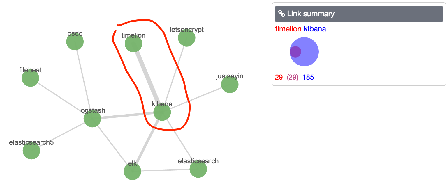
Note how the connections are described using the relative (zero-based) instance number of the vertices. You can also see that the width of a connection is based on the weight (calculated from the significant terms algorithm), rather than document count. Compare the connection width of timelion/kibana (vertices 1 and 5 respectively), with a weighting of 0.33 (kibana -> timelion) and 0.045 (timelion -> kibana) but overlapping document count of 29:

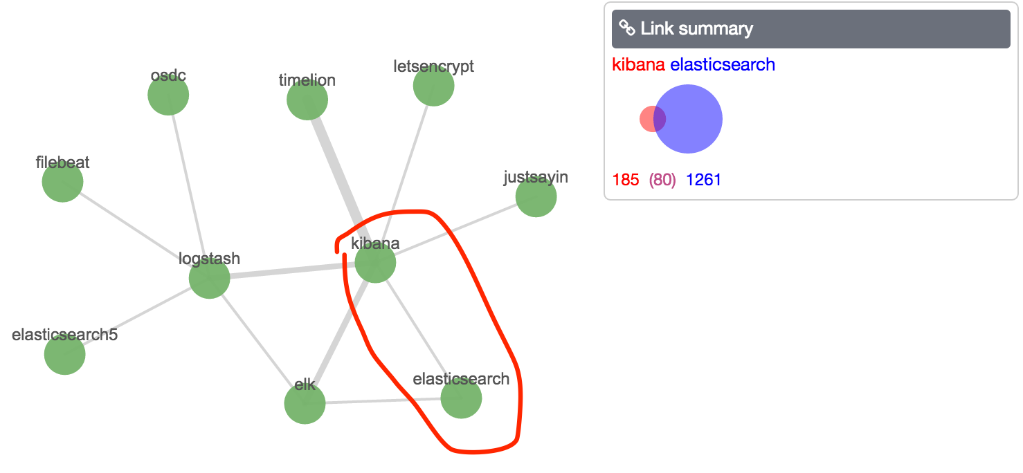
with elasticsearch -> kibana that has an overlapping document count of 80 but only a weight of 0.0001.

Elasticsearch's documentation describes the significant terms algorithm thus, using the example of suggesting "H5N1" when users search for "bird flu" in text:

In all these cases the terms being selected are not simply the most popular terms in a set. They are the terms that have undergone a significant change in popularity measured between a foreground and background set. If the term "H5N1" only exists in 5 documents in a 10 million document index and yet is found in 4 of the 100 documents that make up a user’s search results that is significant and probably very relevant to their search. 5/10,000,000 vs 4/100 is a big swing in frequency.

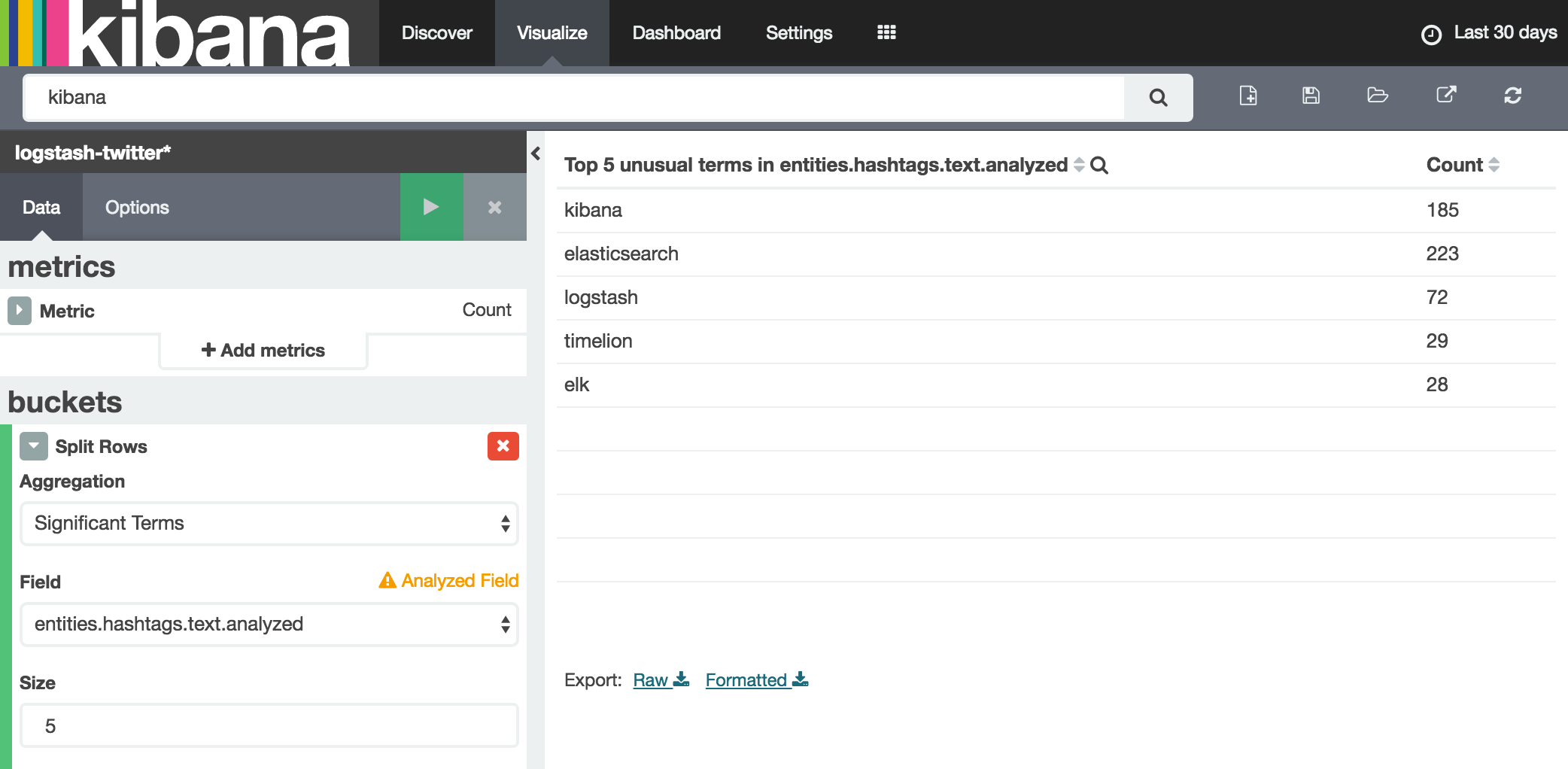
So from this, we can roughly say that Graph is looking at the number of documents in which timelion is mentioned as a proportion of the whole dataset, and then in the number of documents in which the hashtag Kibana exists and also timelion is mentioned. Since the former is a plugin of the latter, the close relationship would be expected. You can use Kibana to explore the significant terms concept further - for example, taking the same 'seed' as the original Graph query above, Kibana, gives a similar set of results as the Graph:

More information about the scoring can be found here, which includes the fact that the scoring is, in part, based on TF-IDF (Term Frequency-Inverse Document Frequency).

Licensing

Graph requires a licence - see here for details.

Conclusion

This tool is a great way to dip one's toe into the waters of Graph analysis and visualisation. It's another approach to consider in the data discovery phase of your analytics work, when you don't even know the questions that you've got for the data in front of you. Your data can remain in Elasticsearch in the same format it's always been, and the Graph function just runs on top of it.

I'll not profess to be a Graph theory expert, so can't pass much comment on the theoretical rigour of the results and techniques seen. One thing that struck me with it was that there's no (apparent) way to manually influence the weight of connections and vertices - for example, based on the number of followers someone has one twitter consider them more (or less) relevant when determining relationships.

For a well-informed view on Graph theory and Social Network Analysis (SNA), see Jordan Meyer's presentation here (and associated R code), as well as Mark Rittman's presentation from BIWA this year.

Footnote: The Twitter Dataset

The dataset I’m using is a live stream from Twitter, via Logstash and Kafka, searching for a set of terms related to me and the field I work in. Therefore, there’s going to be a bunch of relationships missing (if I’ve not included the relevant term in my tweet search), and relationships over-stated (because as a proportion of all the records the terms I’ve selected will dominate).
An interesting use of Graph (or Elasticsearch's significant terms aggregation in general) could be to identify all the relevant terms that I should be including in my twitter search, by sampling an ‘unpolluted’ feed for relationships. For example, if I’m interested in capturing Kafka tweets, perhaps I should also be capturing those related to Samza, Spark, and so on.