Using SparkSQL and Pandas to Import Data into Hive and Big Data Discovery

Big Data Discovery (BDD) is a great tool for exploring, transforming, and visualising data stored in your organisation’s Data Reservoir. I presented a workshop on it at a recent conference, and got an interesting question from the audience that I thought I’d explore further here. Currently the primary route for getting data into BDD requires that it be (i) in HDFS and (ii) have a Hive table defined on top of it. From there, BDD automagically ingests the Hive table, or the data_processing_CLI is manually called which prompts the BDD DGraph engine to go and sample (or read in full) the Hive dataset.

This is great, and works well where the dataset is vast (this is Big Data, after all) and needs the sampling that DGraph provides. It’s also simple enough for Hive tables that have already been defined, perhaps by another team. But - and this was the gist of the question that I got - what about where the Hive table doesn’t exist already? Because if it doesn’t, we now need to declare all the columns as well as choose the all-important SerDe in order to read the data.

SerDes are brilliant, in that they enable the application of a schema-on-read to data in many forms, but at the very early stages of a data project there are probably going to be lots of formats of data (such as TSV, CSV, JSON, as well as log files and so on) from varying sources. Choosing the relevant SerDe for each one, and making sure that BDD is also configured with the necessary jar, as well as manually listing each column to be defined in the table, adds overhead to the project. Wouldn’t it be nice if we could side-step this step somehow? In this article we’ll see how!

Importing Datasets through BDD Studio

Before we get into more fancy options, don’t forget that BDD itself offers the facility to upload CSV, TSV, and XLSX files, as well as connect to JDBC datasources. Data imported this way will be stored by BDD in a Hive table and ingested to DGraph.

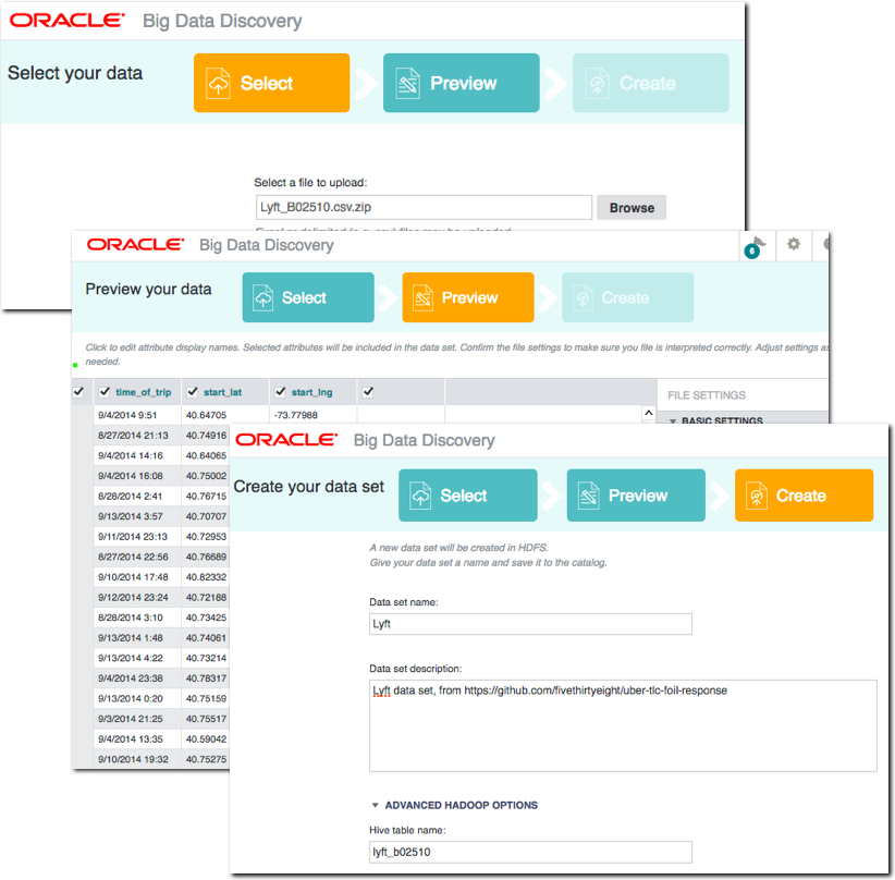
This is great for smaller files held locally. But what about files on your BDD cluster, that are too large to upload from local machine, or in other formats - such as JSON?

Loading a CSV file

As we’ve just seen, CSV files can be imported to Hive/BDD directly through the GUI. But perhaps you’ve got a large CSV file sat local to BDD that you want to import? Or a folder full of varying CSV files that would be too time-consuming to upload through the GUI one-by-one?

For this we can use BDD Shell with the Python Pandas library, and I’m going to do so here through the excellent Jupyter Notebooks interface. You can read more about these here and details of how to configure them on BigDataLite 4.5 here. The great thing about notebooks, whether Jupyter or Zeppelin, is that I don’t need to write any more blog text here - I can simply embed the notebook inline and it is self-documenting:

https://gist.github.com/76b477f69303dd8a9d8ee460a341c445

(gist link)

Note that at end of this we call data_processing_CLI to automatically bring the new table into BDD’s DGraph engine for use in BDD Studio. If you’ve got BDD configured to automagically add new Hive tables, or you don’t want to run this step, you can just comment it out.

Loading simple JSON data

Whilst CSV files are tabular by definition, JSON records can contain nested objects (recursively), as well as arrays. Let’s look at an example of using SparkSQL to import a simple flat JSON file, before then considering how we handle nested and array formats. Note that SparkSQL can read datasets from both local (file://) storage as well as HDFS (hdfs://):

https://gist.github.com/8b7118c230f34f7d57bd9b0aa4e0c34c

(gist link)

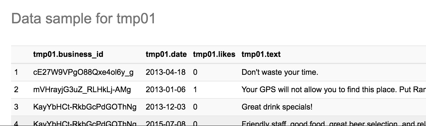
Once loaded into Hive, it can be viewed in Hue:

Loading nested JSON data

What’s been great so far, whether loading CSV, XLS, or simple JSON, is that we’ve not had to list out column names. All that needs modifying in the scripts above to import a different file with a different set of columns is to change the filename and the target tablename. Now we’re going to look at an example of a JSON file with nested objects - which is very common in JSON - and we’re going to have to roll our sleeves up a tad and start hardcoding some schema details.

First up, we import the JSON to a SparkSQL dataframe as before (although this time I’m loading it from HDFS, but local works too):

df = sqlContext.read.json('hdfs:///user/oracle/incoming/twitter/2016/07/12/')

Then I declare this as a temporary table, which enables me to subsequently run queries with SQL against it

df.registerTempTable("twitter")

A very simple example of a SQL query would be to look at the record count:

result_df = sqlContext.sql("select count(*) from twitter")  
result_df.show()

+----+  
| _c0|  
+----+  
|3011|  
+----+

The result of a sqlContext.sql invocation is a dataframe, which above I’m assigning to a new variable, but I could as easily run:

sqlContext.sql("select count(*) from twitter").show()

for the same result.

The sqlContext has inferred the JSON schema automagically, and we can inspect it using

df.printSchema()

The twitter schema is huge, so I’m just quoting a few choice sections of it here to illustrate subsequent points:

root  
|-- created_at: string (nullable = true)  
|-- entities: struct (nullable = true)  
|    |-- hashtags: array (nullable = true)  
|    |    |-- element: struct (containsNull = true)  
|    |    |    |-- indices: array (nullable = true)  
|    |    |    |    |-- element: long (containsNull = true)  
|    |    |    |-- text: string (nullable = true)  
|    |-- user_mentions: array (nullable = true)  
|    |    |-- element: struct (containsNull = true)  
|    |    |    |-- id: long (nullable = true)  
|    |    |    |-- id_str: string (nullable = true)  
|    |    |    |-- indices: array (nullable = true)  
|    |    |    |    |-- element: long (containsNull = true)  
|    |    |    |-- name: string (nullable = true)  
|    |    |    |-- screen_name: string (nullable = true)  
|-- source: string (nullable = true)  
|-- text: string (nullable = true)  
|-- timestamp_ms: string (nullable = true)  
|-- truncated: boolean (nullable = true)  
|-- user: struct (nullable = true)  
|    |-- followers_count: long (nullable = true)  
|    |-- following: string (nullable = true)  
|    |-- friends_count: long (nullable = true)  
|    |-- name: string (nullable = true)  
|    |-- screen_name: string (nullable = true)

Points to note about the schema:

• In the root of the schema we have attributes such as text and created_at
• There are nested elements (“struct”) such as user and within it screen_name, followers_count etc
• There’s also array objects, where an attribute can occur more than one, such as hashtags, and user_mentions.

Accessing root and nested attributes is easy - we just use dot notation:

sqlContext.sql("SELECT created_at, user.screen_name, text FROM twitter").show()

+--------------------+--------------+--------------------+  
|          created_at|   screen_name|                text|  
+--------------------+--------------+--------------------+  
|Tue Jul 12 16:13:...|  Snehalstocks|"Students need to...|  
|Tue Jul 12 16:13:...|   KingMarkT93|Ga caya :( https:...|

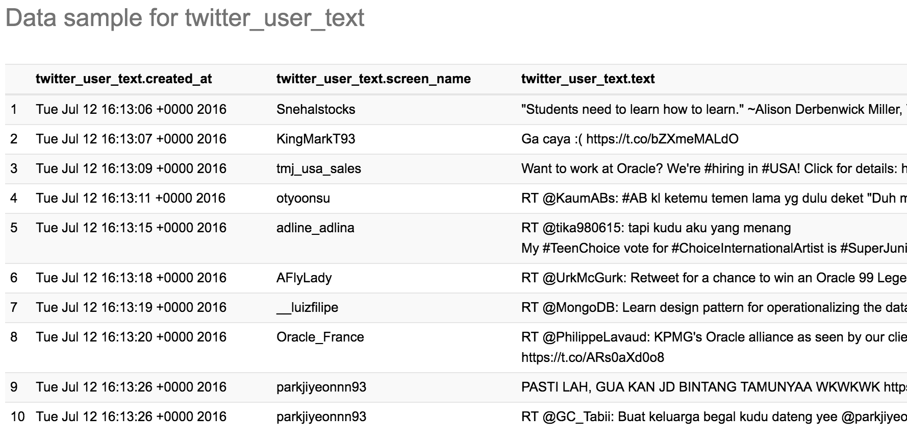
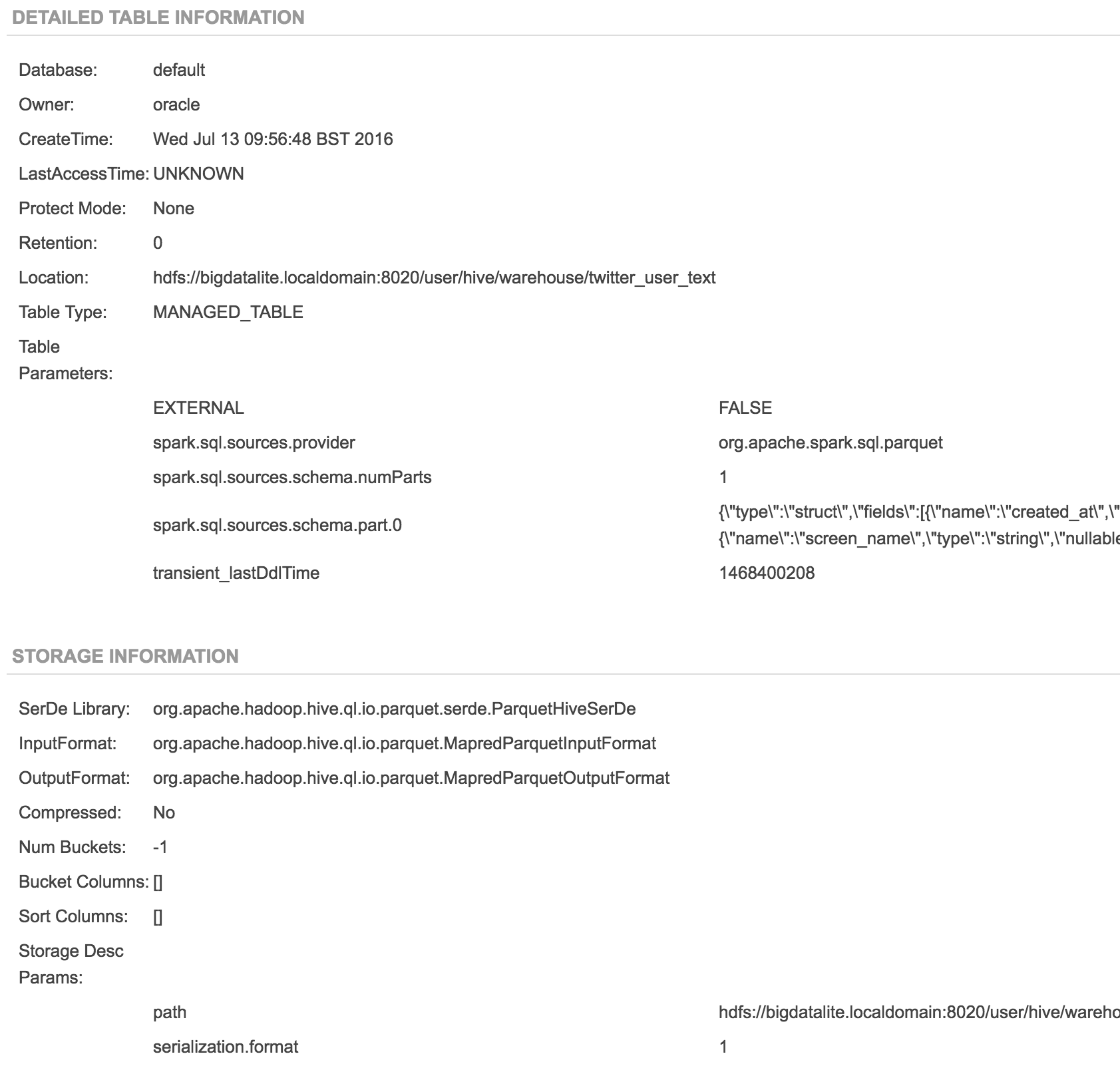
We can save this as a dataframe that’s then persisted to Hive, for ingest into BDD:

subset02 = sqlContext.sql("SELECT created_at, user.screen_name, text FROM twitter")  
tablename = 'twitter_user_text'  
qualified_tablename='default.' + tablename  
subset02.write.mode('Overwrite').saveAsTable(qualified_tablename)

Which in Hue looks like this:

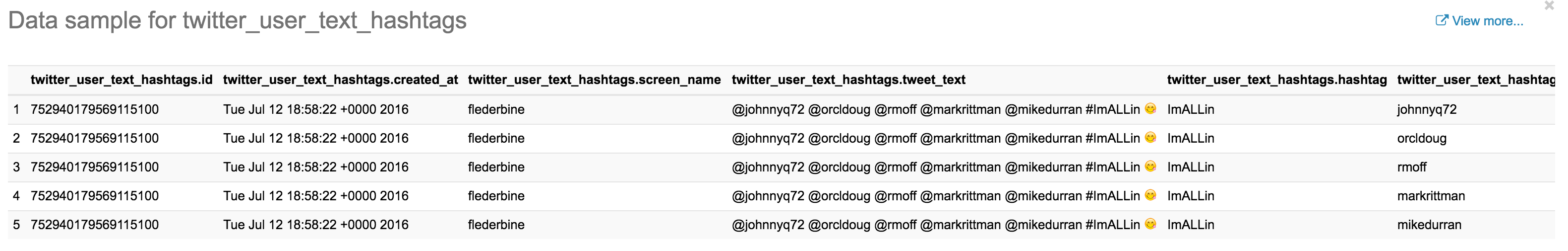
Attributes in an array are a bit more tricky. Here’s an example tweet with multiple user_mentions and a hashtag too:

https://twitter.com/flederbine/status/752940179569115136

Here we use the LATERAL VIEW syntax, with the optional OUTER operator since not all tweets have these additional entities, and we want to make sure we show all tweets including those that don’t have these entities. Here’s the SQL formatted for reading:

SELECT id,  
created_at,  
user.screen_name,  
text as tweet_text,  
hashtag.text as hashtag,  
user_mentions.screen_name as mentioned_user  
from twitter  
LATERAL VIEW OUTER explode(entities.user_mentions) user_mentionsTable as user_mentions  
LATERAL VIEW OUTER explode(entities.hashtags) hashtagsTable AS hashtag

Which when run as from sqlContext.sql() gives us:

+------------------+--------------------+---------------+--------------------+-------+---------------+  
|                id|          created_at|    screen_name|          tweet_text|hashtag|    screen_name|  
+------------------+--------------------+---------------+--------------------+-------+---------------+  
|752940179569115136|Tue Jul 12 18:58:...|     flederbine|@johnnyq72 @orcld...|ImALLin|      johnnyq72|  
|752940179569115136|Tue Jul 12 18:58:...|     flederbine|@johnnyq72 @orcld...|ImALLin|       orcldoug|  
|752940179569115136|Tue Jul 12 18:58:...|     flederbine|@johnnyq72 @orcld...|ImALLin|          rmoff|  
|752940179569115136|Tue Jul 12 18:58:...|     flederbine|@johnnyq72 @orcld...|ImALLin|    markrittman|  
|752940179569115136|Tue Jul 12 18:58:...|     flederbine|@johnnyq72 @orcld...|ImALLin|     mikedurran|  
+------------------+--------------------+---------------+--------------------+-------+---------------+

and written back to Hive for ingest to BDD:

You can use these SQL queries both for simply flattening JSON, as above, or for building summary tables, such as this one showing the most common hashtags in the dataset:

sqlContext.sql("SELECT hashtag.text,count(*) as inst_count from twitter  LATERAL VIEW OUTER explode(entities.hashtags) hashtagsTable AS hashtag GROUP BY hashtag.text order by inst_count desc").show(4)

+-----------+----------+  
|       text|inst_count|  
+-----------+----------+  
|     Hadoop|       165|  
|     Oracle|       151|  
|        job|       128|  
|    BigData|       112|

You can find the full Jupyter Notebook with all these nested/array JSON examples here:

https://gist.github.com/a38e853d3a7dcb48a9df99ce1e3505ff

(gist link)

You may decide after looking at this that you’d rather just go back to Hive and SerDes, and as is frequently the case in ‘data wrangling’ there’s multiple ways to achieve the same end. The route you take comes down to personal preference and familiarity with the toolsets. In this particular case I'd still go for SparkSQL for the initial exploration as it's quicker to 'poke around' the dataset than with defining and re-defining Hive tables -- YMMV. A final point to consider before we dig in is that SparkSQL importing JSON and saving back to HDFS/Hive is a static process, and if your underlying data is changing (e.g. streaming to HDFS from Flume) then you would probably want a Hive table over the HDFS file so that it is live when queried.

Loading an Excel workbook with many sheets

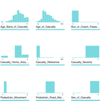
This was the use-case that led me to researching programmatic import of datasets in the first place. I was doing some work with a dataset of road traffic accident data, which included a single XLS file with over 30 sheets, each a lookup table for a separate set of dimension attributes. Importing each sheet one by one through the BDD GUI was tedious, and being a lazy geek, I looked to automate it.

Using Pandas read_excel function and a smidge of Python to loop through each sheet it was easily done. You can see the full notebook here:

https://gist.github.com/rmoff/3fa5d857df8ca5895356c22e420f3b22

(gist link)