Using Partitioning to Improve the Performance of Oracle OLAP Aggregation
When you work with the OLAP Option to Oracle Database 10g, the three things that have the biggest impact on the time it takes to rollup your cube are:
- The order in which you list your dimensions
- How you handle sparsity, and
- How you partition the cube
In the presentation I gave at the Desktop Conference 2006, I thought I handled the "dimension listing" issue fairly well, but I wasn't too happy about how I handled sparsity and partitioning. Sparsity handling, or at least working out whether a dimension is dense or sparse, is a lot easier in 10g Release 2 as there's now a PL/SQL procedure you can use that will work out which dimensions are sparse and which aren't (a future release of AWM will provide a GUI for this). As for partitioning though, I only glossed over this as I wasn't aware at the time that it was so important. As I'm presenting the paper again at Collaborate'06 (probably again with an audience of about 2) I thought I'd look at these two areas again and expand a bit on them. I'll start off by looking at partitioning.
If you're used to doing relational data warehousing using Oracle 8i, 9i or 10g, you'll be familiar with the concept of partitioning. Partitioning lets you split otherwise big tables into lots of little sub-tables, which appear to the user still as a single table, but allow you in the background to place them all on different disk units, load data into individual partitions by using a DDL "trick", back them up and restore them independently, rebuild indexes on them in isolation and so on. Partitioning makes dealing with very large tables a lot easier, and has the potential to make both loading and querying large tables a lot more efficient.
There's a similar concept when you work with analytic workspaces. If you've licensed and installed the Partitioning Option, you can physically partition the table that contains your AW so that individual rows - which in Oracle Database 10g and above, correspond to individual objects in the AW, and before that, correspond to either the whole AW, or chunks of it if it went over a certain segment size - are stored in different partitions, which in turn can be stored in separate tablespaces and datafiles. If you're using 10g or higher and you've got partitioning installed, the OLAP Option creates AWs partitioned by default, albeit with all partitions going into the same tablespace.
Apart from physical partitioning though, release 10.1 of Oracle OLAP brought in a new concept called Logical Partitioning, where you can choose a dimension, hierarchy and level, and partition a measure by this level in order to split it into multiple AW objects. This does not require the partitioning option in the database (but if used in conjunction with it, allows you to put these AW objects into separate physical partitions) and provides the following advantages:
- Just like normal table partitioning, it improves scalability by keeping your data structures small - each partition acts like a smaller measure
- Again, like normal tables, partitioning your measures keeps your working set of data smaller
- It allows your cube build to take advantage of more than one CPU. AWM and the AW/XML Java API that it uses parallelises at the granularity of a partition, and therefore if you've got 4 or 16 CPUs, you'll need to make sure that you've got at least 4 or 16 logical partitions to be able to take advantage of these extra processors. If you don't partition your measures, only one CPU will be used during cube maintenance.
- If you're using the Multi-Write feature in 10g, logical partitioning allows you to have separate sessions updating their own partitions. If you don't partition, only one process will be able to attach and aquire at a time.
- Again, like partitioned tables, you can drop old data and add new data without disturbing existing data.
- If you use compression (compressed composites), aggregation happens at the partition level, such that only those partitions that have new or changed data will be aggregated. This can significantly reduce the time it takes to load in new and changed data.
- Data fragmentation is minimised, as each partition has it's own page of data, and removing for example one month of data won't leave lots of gaps in the remaining data.
So how do you logically partition your cube? Remember, what we're talking about here isn't table partitioning, it's something internal to Oracle OLAP that provides a similar function, but that can be used alongside regular table partitioning if you've paid for this additional database option. So, here's the steps.
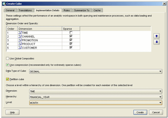
Working with the same cube that I used in the Desktop Conference 2006 paper, you create your cube as normal (it can be in the same analytic workspace as a non-partitioned cube), but when you come to specify the Implementation Details, select "Partition Cube" and choose the dimension, hierarchy and level to partition on, like this:

The question then becomes, which dimension, hierarchy and level do you partition on? As you would expect, there isn't a single "one size fits all" answer to this as there's several factors to bear in mind.
First of all, unlike regular table partitioning, logical partitioning of measures is something that improves the performance of cube loading and aggregation, not querying. In fact, it can actually slow down your queries, and here's why.
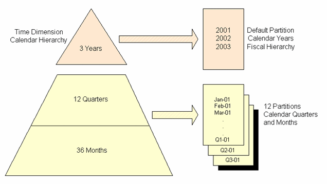
When you partition, for example, by quarter, what the OLAP Option then does is create a separate "partition" variable for each of the quarters in the time dimension, so that for example if you've got three years of data, there'll be twelve partitions that hold measure data, one for each quarter. Then, another, "default" partition is created, that holds all the measure data for any other hierarchies within the time dimension, and any levels above quarter, as illustrated in this diagram from the OLAP Application Developers' Guide:

Now the twist here is that this default partition, often referred to as the "Capstone" partition, doesn't get pre-summarised, i.e. it's values are calculated on the fly. When you come to request measure values that are held in this capstone partition, you're not going to benefit from any pre-summarisation you've done, and the query performance hit when using partitioning, especially when partitioning on a lower-level dimension hierarchy level such as month, can be significant. You may wish to bear this in mind, and either partition on a higher level in the hierarchy, reducing the number of partitions and therefore the scope for parallel aggregation, but ensuring that more of your data is pre-summarised (you can in fact partition on the top, year, level, but again this will limit even more the scope for parallelising your aggregation).
Also, it's not always appropriate to partition on the time dimension. Partitioning on time is useful for a full cube build as you'll be able to split the cube into months or quarters, and spread the load over multiple CPUs, and when you then come to load an individual month or quarter, only the new partition will require aggregation (assuming you're using compressed composites). In some circumstances though, it may make more sense to partition on product group, or geographic district, if this will increase the scope for aggregating in parallel, and there's another instance where this may come in useful; if you've got multiple users updating the cube at the same time, using the multi-write feature in 10g, partitioning by district or product group will mean they can update their own districts or product groups at the same time as other users update their own.
There's a few things to watch out for when you start to use partitioning.
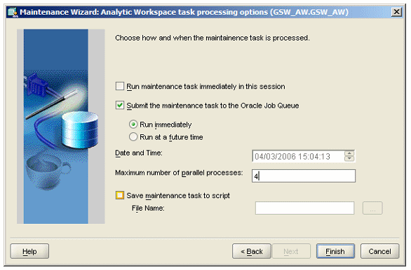
Firstly, even if you define multiple partitions for your cube, Oracle OLAP will only parallelise the aggregation if you submit the maintenance job to the job queue, i.e. don't just run it then and there from AWM10g. This is because, by default, AWM only runs a single process when maintaining a cube, whilst the job queue that AWM uses has the facility to kick off multiple concurrent processes. If you're using AWM, make sure you tick the "Submit the maintenance task to the Oracle Job Queue" tickbox and specify a value >1 for the "Maximum number of parallel processes".

Also, bear in mind that when AWM talks about parallel processes, it's not talking about parallel query, slaves and so on that you get when running regular DML in parallel - what it's referring to here is multiple Oracle sessions running concurrently.
Another thing to bear in mind is that, if you want the aggregation to run in parallel, you need to make sure the "Use Global Composites" box is left unticked - global composites can't be updated in parallel by separate concurrent sessions and you'll need to use the default, local composites instead. If you're using local composites though, it's good if you can try and make it so that individual tuples - combinations of dimension values within the composite - are only found in individual local composites, otherwise you'll find that each of the local composites contains all of the tuples that the other composites contain, although if this happens, the increase in disk space needed is well outweighed by the improvement in aggregation performance.
Also, watch out if you're using partitions with 10g Release 1 - there's a number of optimisations in the aggregation routine used by AWM that are lost if you partition your cube. If you want to use partitioning, it's best to wait until you're on 10g Release 2 because of this issue.
The only other issue is one you might encounter if you partition at too low a level in your hierarchy. If you've got thousands of products that roll up into product groups and product categories, you could well end up with an unmanageable amount of partitions, and you're going to lose the chance to pre-summarise at these higher levels. In this case, it's probably best to partition at a higher level, or choose a dimension such as time for the reasons given above.
Finally, as I mentioned earlier, you can combine this logical cube partitioning with regular table partitioning. By default, if the Partitioning Option is enabled, Analytic Workspaces in Oracle Database 10g have eight physical partitions, but you can increase this number at the time you first create the analytic workspace (this only works if you create the AW manually, rather than using AWM)
SQL> exec dbms_aw.execute('aw create gsw_aw.orders_aw partitions 60');
Creating extra partitions in this way can help improve performance if you've got lots of users concurrently accessing the data, or you want to spread the data over several disks in order to maximise I/O throughput.
As usual, any experiences with logical partitioning are welcomed, and if I've got any bit of this wrong or missed any bit out, let me know and I'll update the article. In the meantime, here's some further reading on partitioning your cubes:
-
Partitioning Large Measures, from the OLAP Application Developers' Guide 10.2
-
Good posting on the OTN OLAP Forum by Chris Chiappa on the typical reasons why a measure gets partitioned
-
Another posting, this time by Dan Peltier, on how 10.2 only aggregates partitions that have been changed, when you use compressed composites
-
Similar posting by "mthompson"
-
Posting by Igor Lubashev on how partitioning is required if you want a measure to be updated by concurrent sessions
-
Posting by myself with an excerpt from a Bud Endress paper on how partitioned variables work in 10g
-
Posting by Jim Carey on how partitioning allows you to use more than one CPU when aggregating (not *the* Jim Carey I presume?)
-
Note from Chris Chiappa on how partitioning can degrade aggregation when using 10.1