More on Oracle OLAP 11g and Query Rewrite

Over the past few days I've been taking a closer look at how query rewrite works with the new 11g release of Oracle OLAP. As a quick recap, in Oracle 11g you can now use OLAP analytic workspaces as summaries within your data warehouse, with Oracle now able to register OLAP dimensions and cubes as "cube organized materialized views", which can be used by the query optimizer as an alternative to regular materialized views. The advantage of using analytic workspaces instead of relational summaries is that a single multi-dimensional analytic workspace can take the place of multiple relational summaries, and an analytic workspace can be faster to aggregate and query than a relational summary.

My interest in this area is mainly due to Discoverer customers asking me over the years whether Oracle OLAP could be a solution to their query performance problems. In the past, whilst moving to an analytic workspace could provide performance benefits when working with large aggregated data sets, you would have had to start using a different version of Discoverer - Oracle Discoverer Plus OLAP - which has a slightly different interface to normal, relational Discoverer, stored it's reports in a different metadata catalog and only had a subset of the functionality of relational Discoverer, albeit with a spiffy new dimensional query builder. Now that the 11g release of Oracle OLAP allows analytic workspaces to be queried just like regular materialized views, it's now possible to use regular Discoverer with it which opens up the possibility of combining the performance of OLAP with the familiarity and maturity of regular SQL-based query tools.

So, my studies followed two main areas: firstly, to see whether Discoverer relational - actually the Windows-based Discoverer Desktop version - can make use of 11g OLAP cubes, and secondly, to take a closer look at how the rewrite process works. To perform the tests, I used the Videostore data set that gets installed in the VIDEO5 schema when you create an End User Layer using Discoverer Administrator, and created an analytic workspace containing measures, dimensions and hierarchies matching the Videostore Discoverer business area.

The Video store data set contains Store, Product and Times dimensions, and a Sales Fact table containing a number of measures.

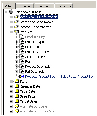
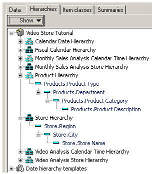
The dimension folders contain items that are arranged into hierarchies, so that users can drill up and drill down in their worksheets.

This more or less translated straight over to an Analytic workspace. A couple of steps that I had to do were firstly, to add a physical “Year” column to the Times table, so that I could create a day > year > all times hierarchy in the analytic workspace – In Discoverer, all of the time dimension attributes are generated at query time using a function, something I usually try and discourage on customer engagements as using a function on the fact table time dimension key can lead to that column’s index not getting used.

The second thing I had to do was to add additional “Total” columns to the Times, Product and Store physical tables, as the analytic workspace would need dimension members at the top level to store measures aggregated up to this top level. If I was building my AW using Oracle Warehouse Builder I could add these additional columns as part of the AW load mapping, but for this example I just added to them to the relational tables and then created the Analytic Workspace.

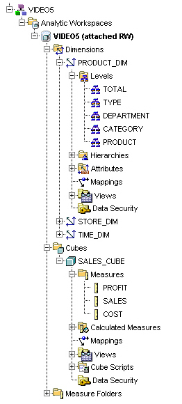
Once I built the Analytic Workspace (which incidentally, I build as a non-partitioned, compressed cube), I removed all of the existing constraints in the VIDEO5 schema and recreated them using the SQL script generated by the Materialized View Advisor, together with some relational dimensions, so that the query optimizer had the best chance of rewriting the queries to use the cube organized materialized views that AWM then generated. Once the Analytic Workspace was created and, using a simple SQL check through SQL Developer, I confirmed that query rewrite against the Analytic Workspace was working, I started my tests.

The first query I ran was a simple table of departments, regions and summarized sales.

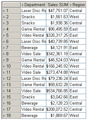
Taking a look at the SQL that Discoverer generated (via the View SQL feature of Discoverer Desktop), it looked like a typical piece of Discoverer SQL.

SELECT O100026.DEPARTMENT, O100028.REGION, SUM(O100027.SALES)
FROM VIDEO5.PRODUCT O100026, VIDEO5.SALES_FACT O100027, VIDEO5.STORE O100028
WHERE ( ( O100026.PRODUCT_KEY = O100027.PRODUCT_KEY ) AND ( O100028.STORE_KEY = O100027.STORE_KEY ) )
GROUP BY O100026.DEPARTMENT, O100028.REGION

Taking a look at the Explain Plan for the query, it looks like it’s been rewritten correctly, now using the cube organized materialized view over the analytic workspace. Moreover, it’s not joined back to the dimensions to get the dimension member names, something it was doing in my previous tests.

SELECT STATEMENT
  HASH GROUP BY
    CUBE SCAN  VIDEO5.CB$SALES_CUBE

So what's happened here in the background is that the Cost-Based Optimizer has decided that, for this particular query block, the analytic workspace (or more precisely, the cube organized materialized view) will return the aggregated data more quickly than the detail-level, relational tables originally specified in the query, so internally it's re-written the query to go to the CB$SALES_CUBE cube organized materialized view. In this particular case, as all of the data it required could be retrieved from the cube organized materialized view - the query just requests what are actually dimension member IDs from the analytic workspace I created - it can get all it needs just from this summary.

Next I put together a crosstab query, to see how that worked.

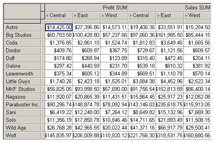
Again, taking a look at the explain plan, it’s been rewritten to use the cube organized materialized view over the Analytic Workspace, but this time I've requested some product data that's actually an attribute in the analytic workspace, as opposed to a dimension member, and so Oracle has had to join back to the dimension tables to get this additional data.

SELECT STATEMENT
  HASH GROUP BY
    HASH JOIN
      CUBE SCAN  VIDEO5.CB$SALES_CUBE
      TABLE ACCESS FULL VIDEO5.PRODUCT

So far, I've just requested aggregated data which the Cost Based Optimized has determined can be most efficiently retrieved from the cube organized materialized view. This materialized view was created using SUM aggregations on the various measures, and contains aggregations for all the combination of product, store and time dimension levels. How, though, would it work if we use an SQL function in our query, say using one of the analytic function worksheets that comes with the Video Store sample data set?

I try it out with the Rank of Sales worksheet.

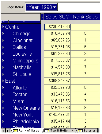
Taking a look at the SQL, you can see the RANK analytic function being used.

SELECT  o100028.CITY as E100089,o100028.REGION as E100106,(decode(o100024.TRANSACTION_DATE,null,to_date(null, 'MMDDYYYY'),to_date(to_char(trunc(o100024.TRANSACTION_DATE,'YYYY'),'YYYY') || '01','YYYYMM'))) as E100200,RANK() OVER(PARTITION BY (decode(o100024.TRANSACTION_DATE,null,to_date(null, 'MMDDYYYY'),to_date(to_char(trunc(o100024.TRANSACTION_DATE,'YYYY'),'YYYY') || '01','YYYYMM'))),o100028.REGION  ORDER BY  ( SUM(o100027.SALES) ) DESC ) as C_1,SUM(o100027.SALES) as E100108_SUM
 FROM VIDEO5.TIMES o100024,
      VIDEO5.SALES_FACT o100027,
      VIDEO5.STORE o100028
 WHERE ( (o100024.TIME_KEY = o100027.TIME_KEY)
   and (o100028.STORE_KEY = o100027.STORE_KEY))
   AND (o100028.REGION IN ('Central','East'))
 GROUP BY o100028.CITY,o100028.REGION,(decode(o100024.TRANSACTION_DATE,null,to_date(null, 'MMDDYYYY'),to_date(to_char(trunc(o100024.TRANSACTION_DATE,'YYYY'),'YYYY') || '01','YYYYMM')));

Again, taking a look at the Explain Plan, it's been re-written to use the cube organized materialized view.

SELECT STATEMENT
  WINDOW SORT
    HASH GROUP BY
      NESTED LOOPS
        NESTED LOOPS
          CUBE SCAN  VIDEO5.CB$SALES_CUBE
          INDEX UNIQUE SCAN VIDEO5.COAD_PK000351
        TABLE ACCESS BY INDEX ROWID VIDEO5.TIMES

Under the covers, the Cost-Based Optimizer has decided that the most efficient way to retrieve sales by city and year, and sales by region and year, is to first go to the cube organized materialized view; then, it uses the SQL engine to perform the ranking, finally returning the results to Discoverer so that it can display the worksheet values. This is exactly the same process that goes on when the query is rewritten to a relational materialized view, with the materialized view providing the summarized data and the SQL engine then ranking it using the WINDOW SORT operation. In this particular case, the query has also had to join back to the dimension tables again to get the year description to use in the worksheet page item.

The only issue I found with rewrite was something, I think, that is a Discoverer-specific issue, in that worksheets that use items taken from a complex folder (one that is made up of arbitrary items dragged into a folder) didn't ever get re-written; I tried out the same query using both regular and complex folders, and whilst the SQL for both queries appeared to be the same, they ended up with different Explain Plans, which I'm guessing is down to some additional hints, joins or something thats actually getting added to queries against complex folders which is stopping re-write occurring. One to check out with an SQL trace at some point.

Whilst we're on the subject of Explain Plans and Oracle OLAP, I was thinking about the SQL statements that my previous "Oracle OLAP and ApEx" posting used; in the example queries I used, I joined individual views over the analytic workspace dimensions and cubes which in the 10g release would have been a pretty inefficient way to query OLAP data - it would have made the OLAP engine return all the dimension records that met the criteria, all the measure records, then have the SQL engine join them before returning the data, which was a bit crazy as the data is already "pre-joined" in the analytic workspace. To get around this issue, the recommended 10g way of accessing analytic workspaces through SQL was to create a single denormalized view over all the dimensions and measures, which whilst being efficient was a bit difficult to work with. In 11g though, there's something called a CUBE JOIN explain plan step that allows you to query analytic workspace views as single items but with the join actually pushed back to the analytic workpace. To see whether this was working, I went back to one of my queries and generated an explain plan.

explain plan for
select
  cu.long_description customer,
  cu.dim_key customer_key,
  cu.parent customer_parent,
  round(f.profit_rank_cust_sh_paren,0) prof_cust_rank_parent,
  round(f.profit_share_cust_sh_pare,1) prof_cust_sh_parent,
  round(f.profit_share_cust_sh_tota,1) prof_cust_sh_level,
  round(f.profit,0) profit,
  round(f.gross_margin,1) gross_margin
FROM time_calendar_view t,
 product_primary_view p,
 customer_shipments_view cu,
 channel_primary_view ch,
 units_cube_view f
WHERE t.level_name = 'CALENDAR_YEAR'
 AND t.calendar_year = 'CY2006'
 AND p.dim_key = 'TOTAL'
 AND cu.parent = 'TOTAL'
 AND ch.dim_key = 'TOTAL'
 AND  t.dim_key = f.time
 AND  p.dim_key = f.product
 AND  cu.dim_key = f.customer
 AND  ch.dim_key = f.channel;
select * from table(dbms_xplan.DISPLAY());
PLAN_TABLE_OUTPUT
Plan hash value: 2133067731

| Id  | Operation                      | Name       | Rows  | Bytes | Cost (%CPU)| Time     |
|   0 | SELECT STATEMENT               |            |    14 |  2338 |    88  (91)| 00:00:02 |

|   1 |  JOINED CUBE SCAN PARTIAL OUTER|            |       |       |            |          |

|   2 |   CUBE ACCESS                  | UNITS_CUBE |       |       |            |          |

|   3 |   CUBE ACCESS                  | CHANNEL    |       |       |            |          |

|   4 |   CUBE ACCESS                  | CUSTOMER   |       |       |            |          |

|   5 |   CUBE ACCESS                  | PRODUCT    |       |       |            |          |

|*  6 |   CUBE ACCESS                  | TIME       |    14 |  2338 |    88  (91)| 00:00:02 |
Predicate Information (identified by operation id):
6 - filter(SYS_OP_ATG(VALUE(KOKBF$),124,125,2)='TOTAL' AND

SYS_OP_ATG(VALUE(KOKBF$),141,142,2)='TOTAL' AND

SYS_OP_ATG(VALUE(KOKBF$),110,111,2)='CY2006' AND

SYS_OP_ATG(VALUE(KOKBF$),112,113,2)='CALENDAR_YEAR' AND

SYS_OP_ATG(VALUE(KOKBF$),155,156,2)='TOTAL' AND SYS_OP_ATG(VALUE(KOKBF$),105,106,2)

IS NOT NULL AND SYS_OP_ATG(VALUE(KOKBF$),124,125,2) IS NOT NULL AND

SYS_OP_ATG(VALUE(KOKBF$),140,141,2) IS NOT NULL AND

SYS_OP_ATG(VALUE(KOKBF$),155,156,2) IS NOT NULL)
25 rows selected

What's happening here is that Oracle is aware that the views I'm querying are actually over an analytic workspace, and it therefore uses the new JOINED CUBE PARTIAL OUTER operation to join the data, passing the joining back to the analytic workspace which does it more efficiently as the data is already joined within its multi-dimensional storage array.

Anyway, it was an interesting bit of studying to do and my thanks also go to Bud Endress from the OLAP Product Management Team for some of the discussions we've had around these new features. Like anything new I'd use it initially with a bit of caution - the cost that the CBO attributes to analytic workspaces compared to regular relational storage is still going through a bit of calibration - but its certainly got some possibilities for Discoverer and other data warehouse setups that need to regularly query large sets of aggregated data, and certainly maintaining a single analytic workspace is a lot less work than maintaining a large set of individual relational summaries. Watch this space for more details as we work through the 11g OLAP release, and if you're interested in working with us on prototyping some of these new features, drop us a line.