OLAP 10gR2 and Dense Looping

Stewart Bryson

Oct 9, 2009 • 9 min read

I'd like to take a moment to express my appreciation to several of the folks at the OLAP product team for their assistance with the project mentioned below, including A.A. Hopeman, Jameson White, Marty Gubar, and especially David Greenfield. The sky's the limit for Oracle OLAP in their capable hands, and I look forward to implementing more projects on 11g in the future.

Recently I completed a project for a client involving an Oracle OLAP implementation in version 10gR2 of the database. The client was developing a reporting solution to plug-in to their proprietary client-server architecture for delivering a content subscription to their customers. Reporting in their application had always been difficult for them, and they decided to deploy Oracle OLAP to ease the maintenance and increase the performance of the reports. The data model and subsequent OLAP model was simple enough... and it seemed like a real match for Oracle OLAP as I looked through the defined dimensions and measures.

One of the reports was especially problematic: the desire to pull back aggregated data according to a custom date range... sometimes that date range was for a particular set of months, other times it was from one individual day to another. To complicate the issue, the report needed to pull back these custom date ranges and display the results across the lowest level of a hierarchy in another dimension. So it wasn't necessarily the custom date range itself that killed the reports, but the fact that this range required data to be pulled back at either the DAY or MONTH level. This coupled with needing to report at the lowest level in an additional hierarchy caused the application to pull back a substantial amount of rows, and Oracle OLAP seemed incapable of doing it in a reasonable amount of time.

In the end, I convinced the client to give version 11g a try to see if some of their performance issues would be alleviated with that release. When it was all done, the performance of 11g was "exponentially faster" to use the client's own words. As a matter of fact, the performance gains were so dramatic that 10g and 11g seemed less like different versions and more like different products all-together.

So I wanted to take a moment to demonstrate a comparable scenario using the SH schema, and view the performance of the same query on the two different database versions: in my case, 10gR2 and 11gR2. When examining some of the timings below, please keep in mind that the Oracle database is running on a virtual machine on my Mac Book Pro, with only 1 virtual CPU and 1 GB of RAM. So it's not the absolute runtimes that concern us, but instead the comparison timings.

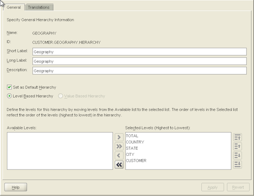
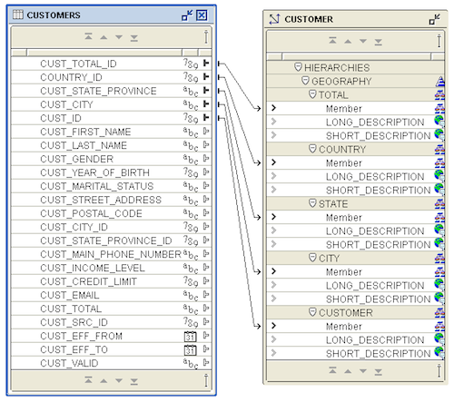
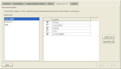
First, I crank up AWM and define the CUSTOMER dimension using surrogate keys, and then define the GEOGRAPHY hierarchy containing the TOTAL, COUNTRY, STATE, CITY and CUSTOMER levels:

Then I use the Mapping Editor to map the relational source, which is the SH.CUSTOMERS table, to the appropriate levels in the CUSTOMER MARKETING hierarchy:

I go on and define the TIME and PRODUCT dimensions in a similar manner. I then build a SALES cube using all three dimensions:

To get the best possible performance in 10gR2, I've enabled compression, and also, to speed up my load times, I've logically partitioned the cube according to the MONTH level in the CALENDAR hierarchy of the TIMES dimension:

Furthermore, I use level-based pre-summarization... the only option in 10gR2. For each hierarchy in the cube, I go through the levels and determine which are to be pre-aggregated and which should be calculated on the fly. The default is to use skip-level aggregation, meaning that every other level level is pre-aggregated, which is a decent trade-off between load performance and query performance. I keep the defaults and move along:

I then map the relational sources to my two measures: QUANTITY_SOLD and AMOUNT_SOLD. These values come from the SALES table in the SH schema:

After I MAINTAIN the cube using AWM, the cube is built, populated and aggregated. I also go on to create the SQL Relational views using the OLAP View Generator plug-in. This allows me to query the SALES cube using simple SQL without having to navigate the complexity of OLAP_TABLE for every single query.

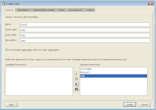
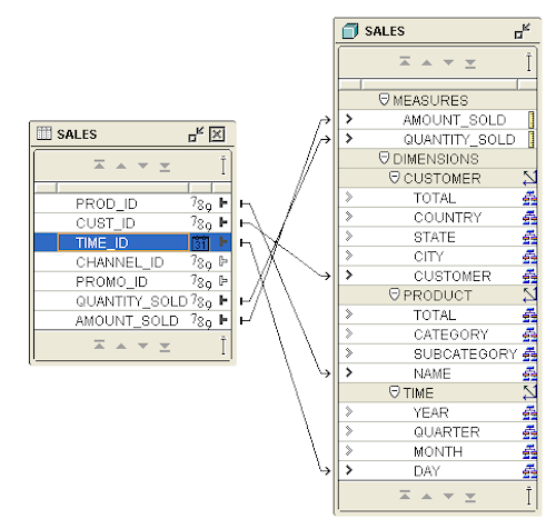
First I query the SALES cube pulling back a small number of rows at pre-aggregated levels. This is the typical use case for Oracle OLAP, and in 10gR2, performs decently. Notice that I'm pulling back CUSTOMER and PRODUCT data at the highest level in the hierarchy, while also pulling data from the TIME dimension at the MONTH level.

SQL> select *
  2    from sh_olap.sales_cubeview
  3   where time_level='MONTH'
  4     and product_level='TOTAL'
  5     and customer_level='TOTAL'
  6     and quantity_sold is not NULL;

48 rows selected.

Elapsed: 00:00:21.96

Execution Plan
----------------------------------------------------------
Plan hash value: 3653525965

------------------------------------------------------------------------------------------------------
| Id  | Operation                           | Name           | Rows  | Bytes | Cost (%CPU)| Time     |
------------------------------------------------------------------------------------------------------
|   0 | SELECT STATEMENT                    |                |     1 | 56092 |    22   (5)| 00:00:01 |
|   1 |  VIEW                               | SALES_CUBEVIEW |     1 | 56092 |    22   (5)| 00:00:01 |
|   2 |   SQL MODEL AW HASH                 |                |     1 |     2 |            |          |
|*  3 |    COLLECTION ITERATOR PICKLER FETCH| OLAP_TABLE     |       |       |            |          |
------------------------------------------------------------------------------------------------------

Predicate Information (identified by operation id):
---------------------------------------------------

   3 - filter(SYS_OP_ATG(VALUE(KOKBF$),30,31,2) IS NOT NULL AND
              SYS_OP_ATG(VALUE(KOKBF$),28,29,2)='MONTH' AND SYS_OP_ATG(VALUE(KOKBF$),19,20,2)='TOTAL' AND
              SYS_OP_ATG(VALUE(KOKBF$),10,11,2)='TOTAL')

Statistics
----------------------------------------------------------
      12264  recursive calls
       1806  db block gets
      23749  consistent gets
       3422  physical reads
        688  redo size
       5082  bytes sent via SQL*Net to client
        392  bytes received via SQL*Net from client
          2  SQL*Net roundtrips to/from client
        295  sorts (memory)
          0  sorts (disk)
         48  rows processed

SQL>

So we pulled 48 rows in 21.96 seconds... not bad for the hardware. But suppose I decide to pull data from CUSTOMER at the individual CUSTOMER level, returning significantly more rows from the cube. Can Oracle OLAP handle it?

SQL> select *
  2    from sh_olap.sales_cubeview
  3   where time_level='MONTH'
  4     and product_level='TOTAL'
  5     and customer_level='CUSTOMER'
  6     and quantity_sold is not NULL;

67034 rows selected.

Elapsed: 00:26:46.94

Execution Plan
----------------------------------------------------------
Plan hash value: 3653525965

------------------------------------------------------------------------------------------------------
| Id  | Operation                           | Name           | Rows  | Bytes | Cost (%CPU)| Time     |
------------------------------------------------------------------------------------------------------
|   0 | SELECT STATEMENT                    |                |     1 | 56092 |    22   (5)| 00:00:01 |
|   1 |  VIEW                               | SALES_CUBEVIEW |     1 | 56092 |    22   (5)| 00:00:01 |
|   2 |   SQL MODEL AW HASH                 |                |     1 |     2 |            |          |
|*  3 |    COLLECTION ITERATOR PICKLER FETCH| OLAP_TABLE     |       |       |            |          |
------------------------------------------------------------------------------------------------------

Predicate Information (identified by operation id):
---------------------------------------------------

   3 - filter(SYS_OP_ATG(VALUE(KOKBF$),30,31,2) IS NOT NULL AND
              SYS_OP_ATG(VALUE(KOKBF$),28,29,2)='MONTH' AND SYS_OP_ATG(VALUE(KOKBF$),19,20,2)='TOTAL' AND
              SYS_OP_ATG(VALUE(KOKBF$),10,11,2)='CUSTOMER')

Statistics
----------------------------------------------------------
        387  recursive calls
     651249  db block gets
   14255252  consistent gets
      12707  physical reads
          0  redo size
    3988723  bytes sent via SQL*Net to client
        535  bytes received via SQL*Net from client
         15  SQL*Net roundtrips to/from client
          0  sorts (memory)
          0  sorts (disk)
      67034  rows processed

SQL>

So returning 67034 rows takes us from a sub-minute query all the way to 26 minutes. Now granted... returning tens of thousands of rows is not typically in the wheelhouse of OLAP. But shouldn't it be? When considering the investment in building and maintaining cubes, it's a real shame if they are incapable of answering all the questions needed for targeted reporting environments.

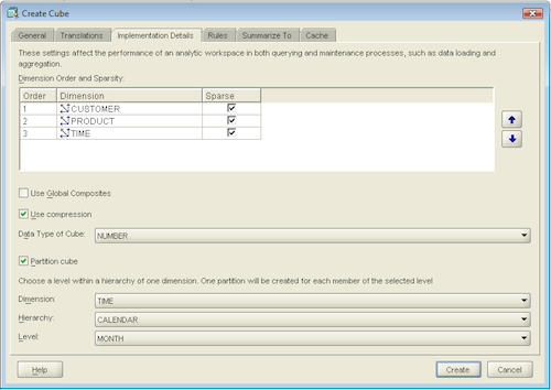
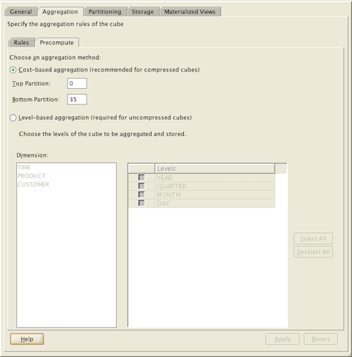
So can 11g do any better? I start up my 11gR2 VM and build the same cube. Significant differences exist between the 10gR2 and 11gR2 versions of AWM, but for the sake of this posting, I'll only point out one: cost-based aggregation, which is only available for compressed cubes. For a more detailed analysis of other differences, see this post and this post by Mark.

Instead of level-based aggregation as we saw above in 10g, we are now able to specify a percentage, which tells the database roughly how many possible cell values at all the different levels in the cube will be pre-calculated. What's more... we are able to dictate different percentages between the top and bottom level partitions.

So let's take a look at the performance we get in 11gR2. The first query is our high-level query, where we are only pulling back values from PRODUCT and CUSTOMER at the TOTAL level, and from TIME at the MONTH level. Notice that the query is slightly different: I actually have to perform a JOIN in the SQL syntax. That's because 11gR2 manages SQL relational views automatically as part of the cube-building process, and they differ somewhat from the ones generated by the AWM plug-in in 10gR2.

SQL> select *
  2    from sh_olap.sales_view c1
  3    JOIN sh_olap.product_view p1 ON product=p1.dim_key
  4    JOIN sh_olap.customer_view c1 ON customer=c1.dim_key
  5    JOIN sh_olap.time_view t1 ON TIME=t1.dim_key
  6   where t1.level_name='MONTH'
  7     and p1.level_name='TOTAL'
  8     and c1.level_name='TOTAL'
  9     and quantity_sold is not null;
48 rows selected.
Elapsed: 00:00:00.11
Execution Plan
Plan hash value: 2133067731

| Id  | Operation         | Name     | Rows  | Bytes | Cost (%CPU)| Time     |
|   0 | SELECT STATEMENT  |          |     1 |   100 |    29   (0)| 00:00:01 |

|   1 |  JOINED CUBE SCAN |          |       |       |            |          |

|   2 |   CUBE ACCESS     | TIME     |       |       |            |          |

|   3 |   CUBE ACCESS     | SALES    |       |       |            |          |

|   4 |   CUBE ACCESS     | CUSTOMER |       |       |            |          |

|*  5 |   CUBE ACCESS     | PRODUCT  |     1 |   100 |    29   (0)| 00:00:01 |
Predicate Information (identified by operation id):
5 - filter(SYS_OP_ATG(VALUE(KOKBF$),2,3,2)='MONTH' AND

SYS_OP_ATG(VALUE(KOKBF$),8,9,2)='TOTAL' AND

SYS_OP_ATG(VALUE(KOKBF$),12,13,2)='TOTAL' AND

SYS_OP_ATG(VALUE(KOKBF$),5,6,2) IS NOT NULL)
Statistics
     10  recursive calls
      0  db block gets
     30  consistent gets
     22  physical reads
      0  redo size
   3526  bytes sent via SQL*Net to client
    349  bytes received via SQL*Net from client
      2  SQL*Net roundtrips to/from client
      1  sorts (memory)
      0  sorts (disk)
     48  rows processed

SQL>

WOW! We just pulled the same 48 rows in only 0.11 seconds. Compared with 22 seconds in 10gR2... 11gR2 is 200 times faster at the high-level query. Now, let's take a look at the more detailed query, where we want to pull values from the CUSTOMER dimension at the CUSTOMER level:

SQL> select *
  2    from sh_olap.sales_view c1
  3    JOIN sh_olap.product_view p1 ON product=p1.dim_key
  4    JOIN sh_olap.customer_view c1 ON customer=c1.dim_key
  5    JOIN sh_olap.time_view t1 ON TIME=t1.dim_key
  6   where t1.level_name='MONTH'
  7     and p1.level_name='TOTAL'
  8     and c1.level_name='CUSTOMER'
  9     and quantity_sold is not null;

67034 rows selected.

Elapsed: 00:00:05.61

Execution Plan
----------------------------------------------------------
Plan hash value: 2133067731

------------------------------------------------------------------------------
| Id  | Operation         | Name     | Rows  | Bytes | Cost (%CPU)| Time     |
------------------------------------------------------------------------------
|   0 | SELECT STATEMENT  |          |     1 |   100 |    29   (0)| 00:00:01 |
|   1 |  JOINED CUBE SCAN |          |       |       |            |          |
|   2 |   CUBE ACCESS     | TIME     |       |       |            |          |
|   3 |   CUBE ACCESS     | SALES    |       |       |            |          |
|   4 |   CUBE ACCESS     | CUSTOMER |       |       |            |          |
|*  5 |   CUBE ACCESS     | PRODUCT  |     1 |   100 |    29   (0)| 00:00:01 |
------------------------------------------------------------------------------

Predicate Information (identified by operation id):
---------------------------------------------------

   5 - filter(SYS_OP_ATG(VALUE(KOKBF$),2,3,2)='MONTH' AND
              SYS_OP_ATG(VALUE(KOKBF$),8,9,2)='TOTAL' AND
              SYS_OP_ATG(VALUE(KOKBF$),12,13,2)='CUSTOMER' AND
              SYS_OP_ATG(VALUE(KOKBF$),5,6,2) IS NOT NULL)

Statistics
----------------------------------------------------------
       2194  recursive calls
       1771  db block gets
       9287  consistent gets
       8183  physical reads
     103152  redo size
    3201497  bytes sent via SQL*Net to client
        492  bytes received via SQL*Net from client
         15  SQL*Net roundtrips to/from client
          9  sorts (memory)
          0  sorts (disk)
      67034  rows processed

SQL>

This query took 26 minutes and 47 seconds on 10gR2, but only 5.61 seconds on 11gR2. The math is staggering... roughly 286 times faster in the new version.

This is not just a newer, faster database (though there is plenty of that as well), but a drastic change in the way 11gR2 retrieves the data from the cube. According to A.A Hopeman from the OLAP product development team at Oracle, the term for this paradigm shift is "LOOP OPTIMIZED":

For 11gR1 we initiated a large project called LOOP OPTIMIZED. This was a coordinated project between the OLAP Engine and the API to have the API produce meta data that lets the engine figure out how to loop as close to "sparsely" (think looping the composite) as possible. This is complex stuff. In 11gR2, the feature is more robust, handles more calc types and is just plain faster. 11gR2 also contains many other features such as improved compression to improve query performance.

David Greenfield, also from the OLAP product team at Oracle, explains what makes LOOP OPTIMIZED performance so much better:

"LOOP OPTIMIZED" improves the way that the AW loops the cube to get results. Suppose, for example, that you have a cube with three dimensions:

TIME: 10 members
PRODUCT: 20 members
CUSTOMER: 30 members

There are 6000 logical cells in this cube (10 * 20 * 30). But your fact will typically have many fewer rows, say 60 for instance. A 'dense loop' of the cube will literally loop all 6000 combinations looking for those 60 cells that have data. A 'sparse loop' of the cube will loop exactly those 60 cells.

The difference in performance between a sparse and dense loop is dramatic.

Dramatic indeed.

Execution Plan

| Id | Operation | Name | Rows | Bytes | Cost (%CPU)| Time |

| 0 | SELECT STATEMENT | | 1 | 100 | 29 (0)| 00:00:01 | | 1 | JOINED CUBE SCAN | | | | | | | 2 | CUBE ACCESS | TIME | | | | | | 3 | CUBE ACCESS | SALES | | | | | | 4 | CUBE ACCESS | CUSTOMER | | | | | |* 5 | CUBE ACCESS | PRODUCT | 1 | 100 | 29 (0)| 00:00:01 |

Predicate Information (identified by operation id):

Statistics

Sign up for more like this.

| 0 | SELECT STATEMENT | | 1 | 100 | 29 (0)| 00:00:01 |
| 1 | JOINED CUBE SCAN | | | | | |
| 2 | CUBE ACCESS | TIME | | | | |
| 3 | CUBE ACCESS | SALES | | | | |
| 4 | CUBE ACCESS | CUSTOMER | | | | |
|* 5 | CUBE ACCESS | PRODUCT | 1 | 100 | 29 (0)| 00:00:01 |