Oracle BI EE 11g - Decoding Essbase Connectivity - Part 1

Venkatakrishnan J

Apr 8, 2011 • 10 min read

If you had gone through my blog series for BI EE 10g and Essbase here, i would have covered the different ways of controlling the BI EE MDX generated for Essbase Sources. With 11g, that too with the introduction of Hierarchical Columns and Value Based Hierarchies, the entire series needs a relook in the context of 11g. So, this blog post is the first in series of BI EE 11g - Essbase connectivity. In this series, we shall be seeing how BI EE 11g generates MDX and how that changes as we start using the various new features of BI EE 11g. I will be using the Essbase 11.1.2 version for all these posts.

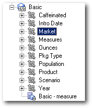
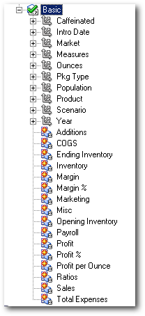
We start off by taking the simple Demo > Basic cube and then importing it to BI EE. We shall be understanding the connectivity by altering 4 main parameters in the Repository. They are

Physical Layer Aggregation (which i will term as PA going forward)
Business Model Layer Aggregation (which i will term as BA going forward)
Hierarchy Type (which i will term as HT going forward)
Measure Type (which i will terms as MT going forward)

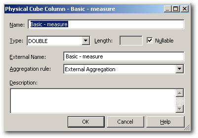
Physical Layer Aggregation:

This is the value that we set for the measures in the physical layer. The default value will be External Aggregation.

Business Model Layer Aggregation:

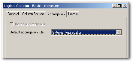
This is the aggregation that we set for measures in the Business Model & Mapping Layer. The default value will be External Aggregation.

Hierarchy Type:

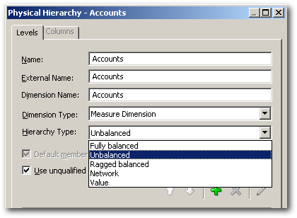
In BIEE 11g, each dimension (for BSO cubes) or each hierarchy (for ASO cubes with multiple hierarchies enabled) can be assigned a hierarchy type. There can be a range of hierarchies that can be assigned. The commonly used ones are Balanced, Unbalanced, Ragged and Value. Changing the hierarchy types can have significant impact on the way MDX is generated.

NewImage

Measure Type:

In BI EE 11g, there are 2 ways to treat measures. One is the default Essbase way where we have a single data measure or a flattened version of the measure hierarchy. This can have a significant impact on the way MDX is generated.

NewImage

With that overview, lets start our first analysis by looking at the kind of MDX that BI EE generates for the most common way of modeling(mostly defaults for all the properties above).

1. PA - External Aggregation, BA - External Aggregation, HT - All dimensions marked as Unbalanced(BSO Cube), MT - Single Measure Essbase Type Model

Using Attribute Columns:

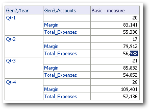
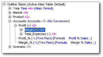
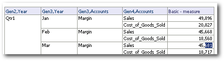
We start off with creating a simple report containing 2 dimensions. One is an Accounts dimension (marked as Measure dimension in Physical layer) and the other is the normal time dimension. The report is shown below

NewImage

Lets now take a look at the MDX for this report.

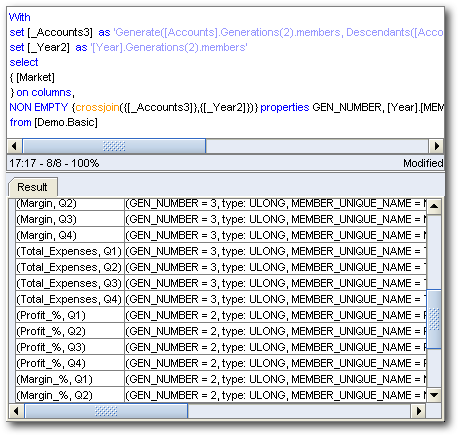
With
set [_Accounts3]  as 'Generate([Accounts].Generations(2).members, Descendants([Accounts].currentmember, [Accounts].Generations(3), leaves))'
set [_Year2]  as '[Year].Generations(2).members'select{ [Market]} on columns,
NON EMPTY {crossjoin({[_Accounts3]},{[_Year2]})}
properties GEN_NUMBER, [Year].[MEMBER_UNIQUE_NAME],
[Year].[Memnor], [Accounts].[MEMBER_UNIQUE_NAME],
[Accounts].[Memnor] on rowsfrom [Demo.Basic]

There are 2 things that we notice immediately from the above report. First one is, since we have made the dimension Accounts as Unbalanced, we get a null value. The reason for this is, our accounts structure is ragged and is not balanced as shown below.

The second thing that we can notice is the MDX itself. Though we have included just Generation 3 of Accounts in the report, it goes all the way down to the lowermost level (Leaves clause in the MDX). So, lets fire this MDX directly in EAS and find out the actual output.

As you see, the MDX extracts the data for all the Leave Members which do not have a Generation 3. So, in the above report Profit_% and Margin_% are combined together for every Time intersection at the BI Server layer. Let's now drill down on the Margin member and see what happens.

Interestingly this generates 2 MDX statements. In 10g, in majority of the cases, there will be only one MDX statement for any report irrespective of the property setting.

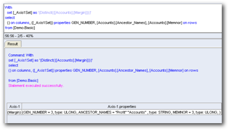
With
set [_Axis1Set] as '{Distinct({[Accounts].[Margin]})}'
select{} on columns, 
{[_Axis1Set]} properties GEN_NUMBER, 
[Accounts].[Ancestor_Names], [Accounts].[Memnor] on rows
from [Demo.Basic]

With
set [_Accounts3]  as '{Distinct({[Accounts].[Margin]})}'set [_Accounts4]  as 'Generate([_Accounts3], 
Descendants([Accounts].currentmember, [Accounts].Generations(4), leaves))'
set [_Year2]  as '{Distinct({[Year].[Qtr1]})}'
select{ [Market]} on columns,
NON EMPTY {crossjoin({[_Accounts4]},{[_Year2]})} 
properties GEN_NUMBER, [Year].[MEMBER_UNIQUE_NAME], 
[Year].[Memnor], [Accounts].[Ancestor_Names], 
[Accounts].[MEMBER_UNIQUE_NAME], [Accounts].[Memnor] on rows
from [Demo.Basic]

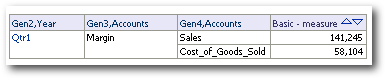
Let's see what each of the above MDX produce in EAS.

NewImage

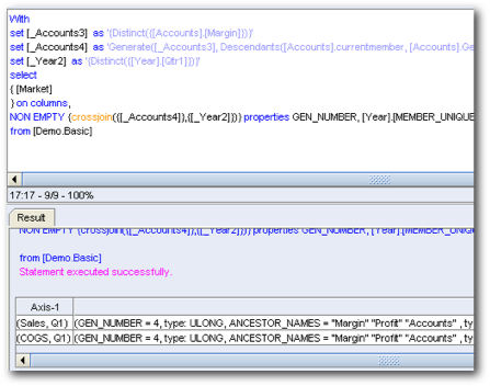
The first MDX basically does a distinct on the Margin member. And the second query gets the data corresponding to those members. This is a big difference between 10g and 11g. The main reason for the new query for enabling the display of reports in outline sort order.

To see whether we are getting a seamless behaviour, lets now drill on Qtr1 in the same report.

NewImage

If we now look at the MDX, there will be 3 separate queries. One for Year, Accounts and then for the actual data itself. This is pretty good and is actually one step forward from 10g.

With
set [_Axis1Set] as '{Distinct({[Year].[Qtr1]})}'
select{} on columns, {[_Axis1Set]} properties GEN_NUMBER, [Year].[Ancestor_Names], 
[Year].[Memnor] on rowsfrom [Demo.Basic]

With
set [_Axis1Set] as '{Distinct({[Accounts].[Margin]})}'select{} on columns, 
{[_Axis1Set]} properties GEN_NUMBER, [Accounts].[Ancestor_Names], [Accounts].[Memnor] on rows
from [Demo.Basic]

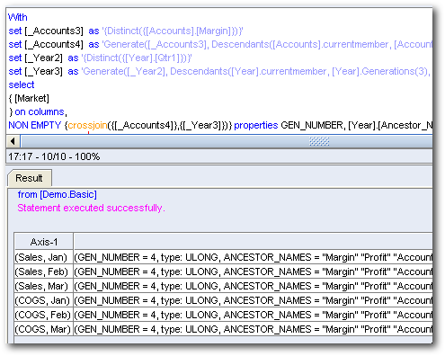
With
set [_Accounts3]  as '{Distinct({[Accounts].[Margin]})}'
set [_Accounts4]  as 'Generate([_Accounts3], Descendants([Accounts].currentmember, [Accounts].Generations(4), leaves))'
set [_Year2]  as '{Distinct({[Year].[Qtr1]})}'
set [_Year3]  as 'Generate([_Year2], Descendants([Year].currentmember, [Year].Generations(3), leaves))'
select{ [Market]} on columns,
NON EMPTY {crossjoin({[_Accounts4]},{[_Year3]})} properties GEN_NUMBER, 
[Year].[Ancestor_Names], [Year].[MEMBER_UNIQUE_NAME], [Year].[Memnor], [Accounts].[Ancestor_Names], [Accounts].[MEMBER_UNIQUE_NAME], [Accounts].[Memnor] on rows
from [Demo.Basic]

Let's now fire the last query in EAS. You can see a significant difference in the output of this query and the final out of the report shown above.

NewImage

The main difference is in the ordering. Till BI EE 10g, by default BI EE sorted the results in alphabetical order. There was no easy way to enable sorting in outline order. Basically with multiple queries, BI EE 11g achieves the outline sorting.

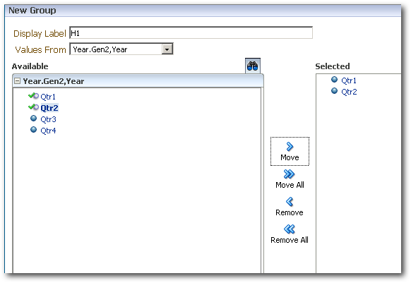
Custom Groups & Selection Steps:

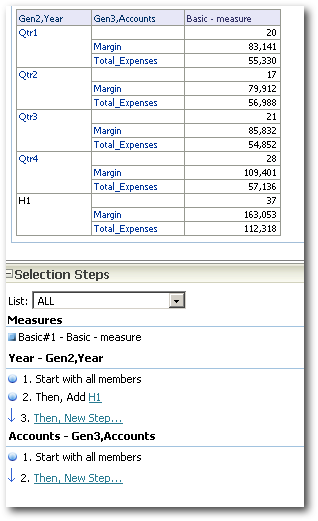
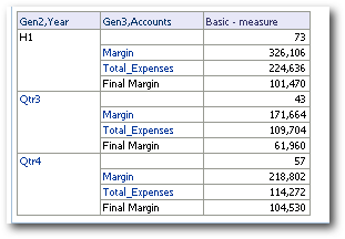
Now that we have seen a basic report and how it behaves, lets look at the new Custom Groups feature of BI EE. Lets now create a Custom Group called H1 which will group Qtr1 and Qtr2 together.

NewImage

As you see, as soon as we added the custom group, we have a custom selection step. Applying multiple Selection Steps will actually change the Logical SQL itself. So, let's take a look at the Logical SQL first before looking at the MDX.

NewImage

As you see, since we added a custom Group H1 to the report, BI EE 11g will push that as a separate MDX (2nd UNION ALL Logical SQL) and will combine that with the main MDX. Let's look at the MDX specific to the custom group alone.

With
set [_Accounts3]  as 'Generate([Accounts].Generations(2).members, 
Descendants([Accounts].currentmember, [Accounts].Generations(3), leaves))'
member [Year].[YearCustomGroup] as '[Year].[Qtr1] + [Year].[Qtr2]', SOLVE_ORDER = AGGREGATION_SOLVEORDER
select{ [Market]} on columns,
NON EMPTY {{[_Accounts3]}} properties GEN_NUMBER, [Accounts].[MEMBER_UNIQUE_NAME], [Accounts].[Memnor] on rows
from [Demo.Basic]where ([Year].[YearCustomGroup])

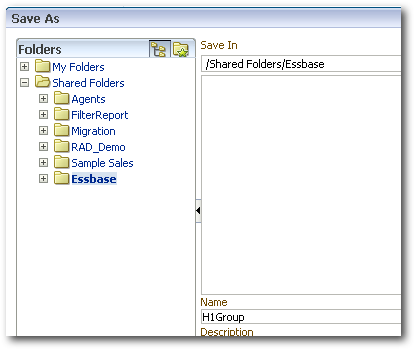
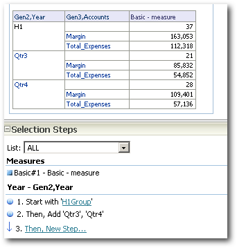
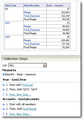
So far so good. As you notice, BI EE has generated a very efficient MDX even for custom Groups. Let's now alter this to report to group Qtr1 & Qtr2 as H1 but display the Qtr3, Qtr4 as is in the same level. To do this, we need to first save the Custom Group we created.

NewImage

Then we need to alter the Selection Steps of the Year dimension as shown below

NewImage

If we look at the Logical SQL, we should see 2 UNION requests as shown below.

NewImage

As you notice, BI EE generates the expected Logical SQL. If we look at the actual MDX generated we should see 2 main (apart from the ones used for sorting) MDX. One for the custom Group and the other for Qtr3 and Qtr4.

With
set [_Accounts3]  as 'Generate([Accounts].Generations(2).members, 
Descendants([Accounts].currentmember, [Accounts].Generations(3), leaves))'
member [Year].[YearCustomGroup] as '[Year].[Qtr1] + [Year].[Qtr2]', SOLVE_ORDER = AGGREGATION_SOLVEORDER
select{ [Market]} on columns,
NON EMPTY {{[_Accounts3]}} properties GEN_NUMBER, [Accounts].[MEMBER_UNIQUE_NAME], [Accounts].[Memnor] on rows
from [Demo.Basic]where ([Year].[YearCustomGroup])

With
set [_Accounts3]  as 'Generate([Accounts].Generations(2).members, 
Descendants([Accounts].currentmember, [Accounts].Generations(3), leaves))'
set [_Year2]  as '{Distinct({[Year].[Qtr3], [Year].[Qtr4]})}'select{ [Market]} on columns,
NON EMPTY {crossjoin({[_Accounts3]},{[_Year2]})} properties GEN_NUMBER, 
[Year].[MEMBER_UNIQUE_NAME], [Year].[Memnor], [Accounts].[MEMBER_UNIQUE_NAME], [Accounts].[Memnor] on rows
from [Demo.Basic]

Both of these are efficient MDX queries. Now let's make the query a little bit more complex and add a Custom Calculation called Final Margin which will be the difference of Margin and Total Expenses.

As you see, there are 4 UNION ALL statements in this query. So, in effect, if we have n dimensions with each dimension having m selection steps, there will in total be n*m MDX queries fired back to the database. Same is the case for even relational sources. Let's now look at the MDX generated.

With
set [_Accounts3]  as 'Generate([Accounts].Generations(2).members, 
Descendants([Accounts].currentmember, [Accounts].Generations(3), leaves))'
member [Year].[YearCustomGroup] as '[Year].[Qtr1] + [Year].[Qtr2]', SOLVE_ORDER = AGGREGATION_SOLVEORDER
select{ [Market]} on columns,NON EMPTY {{[_Accounts3]}} properties GEN_NUMBER, 
[Accounts].[MEMBER_UNIQUE_NAME], [Accounts].[Memnor] on rows
from [Demo.Basic]
where ([Year].[YearCustomGroup])

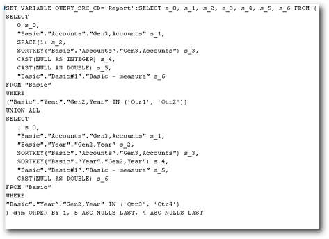
With
set [_Accounts3]  as '{Distinct({[Accounts].[Margin], [Accounts].[Total_Expenses]})}'
set [_Year2]  as '{Distinct({[Year].[Qtr1], [Year].[Qtr2]})}'select{ [Market]} on columns,
NON EMPTY {crossjoin({[_Accounts3]},{[_Year2]})} properties GEN_NUMBER, 
[Year].[MEMBER_UNIQUE_NAME], [Year].[Memnor], [Accounts].[MEMBER_UNIQUE_NAME], 
[Accounts].[Memnor] on rows
from [Demo.Basic]

With
set [_Accounts3]  as 'Generate([Accounts].Generations(2).members,
Descendants([Accounts].currentmember, [Accounts].Generations(3), leaves))'
set [_Year2]  as '{Distinct({[Year].[Qtr3], [Year].[Qtr4]})}'select{ [Market]} on columns,
NON EMPTY {crossjoin({[_Accounts3]},{[_Year2]})} properties GEN_NUMBER, 
[Year].[MEMBER_UNIQUE_NAME], [Year].[Memnor], [Accounts].[MEMBER_UNIQUE_NAME], 
[Accounts].[Memnor] on rowsfrom [Demo.Basic]

With
set [_Accounts3]  as '{Distinct({[Accounts].[Margin], [Accounts].[Total_Expenses]})}'
set [_Year2]  as '{Distinct({[Year].[Qtr3], [Year].[Qtr4]})}'select{ [Market]} on columns,
NON EMPTY {crossjoin({[_Accounts3]},{[_Year2]})} properties GEN_NUMBER, 
[Year].[MEMBER_UNIQUE_NAME], [Year].[Memnor], [Accounts].[MEMBER_UNIQUE_NAME], 
[Accounts].[Memnor] on rows
from [Demo.Basic]

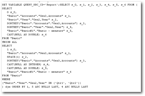
By looking at this we can notice 3 important things

Custom Group with normal Dimension filter pushes the grouping operation directly within MDX - Query 1 in the list of 4 queries above.
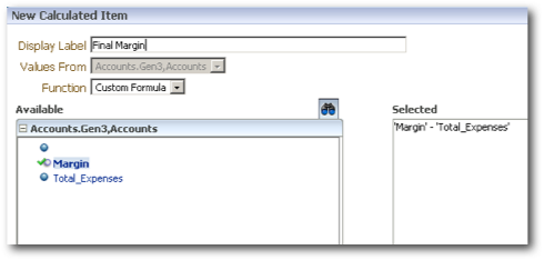
A custom calculation does not get converted into a physical MDX. Rather it is always done at the BI EE layer - Query 2 & 4 of the 4 queries above.
A custom Group when combined with a custom Calculation, the MDX fired is at the base level without the calculations. The calculation is done by the BI Server instead - Query 4 above.

The above 3 observations are very important as these can determine the performance of the final report generated.

BI Server Calculation Functions:

Another important part to test is the ability of the BI server to apply custom functions on any data source. MDX inherently does not support quite a lot of string functions (like add a prefix to a member etc). In those cases, BI server processing can come in handy. In 10g, whenever PA is Aggr_External and BA is Aggr_External we cannot apply BI Server functions as 10g did not have the capability to function ship many of the functions back to Essbase. So let's put that to test in 11g (we are in case 1 where PA is External Aggregation {Aggr_External in 10g} and BA is External Aggregation).

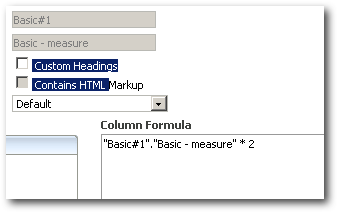
To the same report let's add a custom function to multiply the measure by say 2.

NewImage

Interesting it pushes the calculation directly to the BI Server (not pushed to Essbase through MDX). This works even when we have the measures externally aggregated. Let's now, put this through one more test. Let's add a prefix to the Gen3, Accounts using the formula below

NewImage

As expected, we still get the dreaded Cannot function ship error message. The last feature to test from the 10g world is the use of Evaluate functions.

EVALUATE Functions:

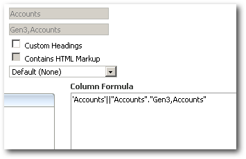
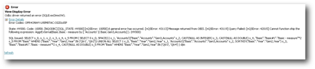
This is one other feature that was used quite a lot in BI EE 10g. Most complex reports created out of BI EE 10g on Essbase would have involved some sort of MDX function. To check whether the EVALUATE works the same way, let's remove all the Selection Steps and then apply a new measure EVALUATE function as shown below.

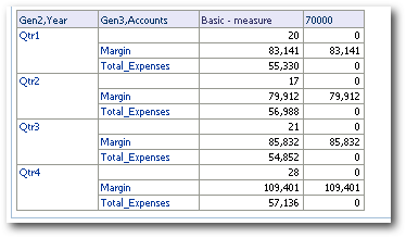
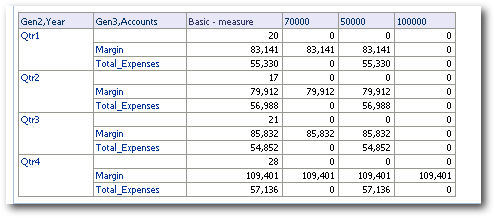
EVALUATE('case when (%1.dimension.currentmember,%2.dimension.currentmember,[Actual]) > 70000 then (%1.dimension.currentmember,%2.dimension.currentmember,[Actual]) else 0 end' AS INTEGER,"Year"."Gen2,Year","Accounts"."Gen3,Accounts")

All this function does is, it basically applies a case when statement on the measure. Whenever the Actual Scenario value is greater than 70000, it will be shown as is else will be shown as is, else will be shown as 0. Lets see how this translates into the report.

NewImage

As you see, it works well. In 10g, there was a bug wherein we could not have more than one EVALUATE function referring the same column. Let's check whether that has been fixed.

NewImage

This is very good. We can now apply multiple EVALUATE functions thereby opening up the connectivity a bit further. In the next post we shall how the MDX gets affected once we start including the Hierarchical Columns.

Sign up for more like this.