Using the ELK Stack to Analyse Donor's Choose Data


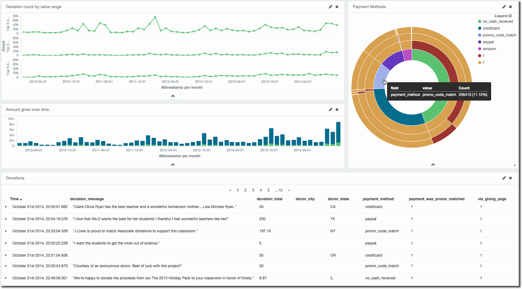
Donor’s Choose is an online charity in America through which teachers can post details of projects that need funding and donors can give money towards them. The data from the charity since it began in 2000 is available to download freely here in several CSV datasets. In this article I'm going to show how to use the ELK stack of data discovery tools from Elastic to easily import some data (the donations dataset) and quickly start analysing it to produce results such as this one:
I’m assuming you’ve downloaded and unzipped Elasticsearch, Logstash and Kibana and made Java available if not already. I did this on a Mac, but the tools are cross-platform and should work just the same on Windows and Linux. I’d also recommend installing Kopf, which is an excellent plugin for the management of Elasticsearch.
CSV Data Ingest with Logstash
First off we’re going to get the data in to Elasticsearch using Logstash, after which we can do some analysis using Kibana.
To import the data with Logstash requires a configuration file which in this case is pretty straightforward. We’ll use the file input plugin, process it with the csv filter, set the date of the event to the donation timestamp (rather than now), cast a few fields to numeric, and then output it using the elasticsearch plugin. See inline comments for explanation of each step:
input {
    file {
        # This is necessary to ensure that the file is
        # processed in full. Without it logstash will default
        # to only processing new entries to the file (as would
        # be seen with a logfile for a live application, but
        # not static data like we're working with here)
        start_position  => beginning
        # This is the full path to the file to process.
        # Wildcards are valid.
        path =>  ["/hdd/ELK/data/opendata/opendata_donations.csv"]
    }
}

filter {
        # Process the input using the csv filter.
        # The list of column names I took manually from the
        # file itself
        csv {separator => ","
                columns => ["_donationid","_projectid","_donor_acctid","_cartid","donor_city","donor_state","donor_zip","is_teacher_acct","donation_timestamp","donation_to_project","donation_optional_support","donation_total","dollar_amount","donation_included_optional_support","payment_method","payment_included_acct_credit","payment_included_campaign_gift_card","payment_included_web_purchased_gift_card","payment_was_promo_matched","via_giving_page","for_honoree","donation_message"]}

        # Store the date of the donation (rather than now) as the
        # event's timestamp
        #
        # Note that the data in the file uses formats both with and
        # without the milliseconds, so both formats are supplied
        # here.
        # Additional formats can be specified using the Joda syntax
        # (http://joda-time.sourceforge.net/api-release/org/joda/time/format/DateTimeFormat.html)
        date { match => ["donation_timestamp", "yyyy-MM-dd HH:mm:ss.SSS", "yyyy-MM-dd HH:mm:ss"]}
        # ------------
        # Cast the numeric fields to float (not mandatory but makes for additional analysis potential)
        mutate {
        convert => ["donation_optional_support","float"]
        convert => ["donation_to_project","float"]
        convert => ["donation_total","float"]
        }
}

output {
        # Now send it to Elasticsearch which here is running
        # on the same machine.
        elasticsearch { host => "localhost" index => "opendata" index_type => "donations"}
        }
With the configuration file created, we can now run the import:
./logstash-1.5.0.rc2/bin/logstash agent -f ./logstash-opendata-donations.conf
This will take a few minutes, during which your machine CPU will rocket as logstash processes all the records. Since logstash was originally designed for ingesting logfiles as they’re created it doesn’t actually exit after finishing processing the file, but you’ll notice your machine’s CPU return to normal, at which point you can hit Ctrl-C to kill logstash.
If you’ve installed Kopf then you can see at a glance how much data has been loaded:

curl -XGET 'http://localhost:9200/opendata/_status?pretty=true'

[...]
    "opendata" : {
      "index" : {
        "primary_size_in_bytes" : 3679712363,
      },
[...]
      "docs" : {
        "num_docs" : 2608803,
Note that Elasticsearch will take more space than the source data (in total the 1.2Gb dataset ends up taking c.5Gb)
Data Exploration with Kibana
Now we can go to Kibana and start to analyse the data. From the Settings page of Kibana add the opendata index that we’ve just created:


- two thirds of donations were in the 10-100 dollar range
- four-fifths included the optional donation towards the running costs of Donor's Choose.


Data Visualisation with Kibana
One of my favourite features of Kibana is its ability to aggregate data at various dimensions and grains with ridiculous ease. Here’s an example: (click to open full size)


Kibana Dashboards
Now let’s bring the visualisations together along with the data table we saw in the the Discover tab. Click on Dashboard, and then the + icon:


Example Analysis
Let's look at some actual data analyses now. One of the most simple is the amount given in donations over time, split by amount given to project and also as the optional support amount:

One of the nice things about Kibana is the ability to quickly change resolution in a graph's time frame. By default a bar chart will use an "Auto" granularity on the time axis, updating as you zoom in and out so that you always see an appropriate level of aggregation. This can be overridden to show, for example, year-on-year changes:

You can also easily switch the layout of the chart, for example to show the percentage of the two aggregations relative to each other. So whilst the above chart shows the optional support amount increasing by the year, it's actually remaining pretty much the same when taken as a percentage of the donations overall - which if you look into the definition of the field ("we encourage donors to dedicate 15% of each donation to support the work that we do.") makes a lot of sense

Analysis based on text in the data is easy. You can use the Terms sub-aggregation, where here we can see the top five states in terms of donation amount, California consistently being the top of the table.

Since the Terms sub-aggregation shows the Top-x only, you can't necessarily judge the importance of those values in relation to the rest of the data. To do this more specific analysis you can use the Filters sub-aggregation to use free-form searches to create buckets, such as here to look at how much those from NY and CA donated, vs all other states. The syntax is field:value to include it, and -field:value to negate it. You can string these expressions together using AND and OR.

A lot of the analysis generally sits well in the bar chart visualisation, but the line chart has a role to play too. Donations are grouped according to the value range (<10, between 10 and 100, > 100), and these plot out nicely when considering the number of donations made (rather than total value). Whilst the total donation in a time period is significant, so is the engagement with the donors hence the number of donations made is important to analyse:

As well as splitting lines and bars, you can split charts themselves, which works well when you want to start comparing multiple dimensions without cluttering up a single chart. Here's the same chart as previously but split out with one line per instance. Arguably it's clearer to understand, and the relative values of the three items can be better seen here than in the clutter of the previous chart:

Following on from this previous graph, I'm interested in the spike in mid-value ($10-$100) donations at the end of 2011. Let's pull the graph onto a dashboard and dig into it a bit. I've saved the visualisation and brought it in with the saved Search (from the Discover page earlier) and an additional visualisation showing payment methods for the donations:

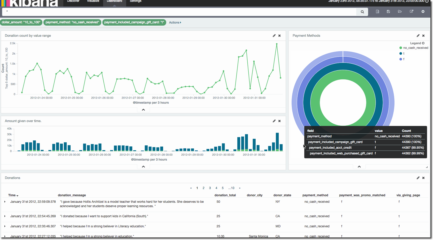
Now I can click and drag the time frame to isolate the data of interest and we see that the number of donations jumps eight-fold at this point:

Clicking on one of the data points drills into it, and we eventually see that the spike was attributable to the use of campaign gift cards, presumably issued with a value > $10 and < $100.

Limitations
The simplicity described in this article comes at a cost, or rather, has its limits. You may well notice fields in the input data such as “_projectid”, and if you wanted to relate a donation to a given project you’d need to go and look that project code up manually. There’s no (easy) way of doing this in Elasticsearch - whilst you can easily bring in all the project data too and search on projectid, you can’t display the two (project and donation) alongside each other (easily). That’s because Elasticsearch is a document store, not a relational database. There are some options discussed on the Elasticsearch blog for handling this, none of which to my mind are applicable to this kind of data discovery (but Elasticsearch is used in a variety of applications, not just as a data store for Kibana, so in others cases it is more relevant). Given that, and if you wanted to resolve this relationship, you’d have to go about it a different way, maybe using the linux join command to pre-process the files and denormalise them prior to ingest with logstash. At this point you reach the “right tool/right job” decision - ELK is great, but not for everything :-)
Reprocessing
If you need to reload the data (for example, when building this I reprocessed the file in order to define the numerics as such, rather than the default string), you need to :
- Drop the Elasticsearch data:
curl -XDELETE 'http://localhost:9200/opendata'
- Remove the “sincedb” file that logstash uses to record where it last read from in a file (useful for tailing changing input files; not so for us with a static input file)
rm ~/.sincedb*
(better here would be to define a bespoke sincedb path in the file input parameters so we could delete a specific sincedb file without impacting other logstash processing that may be using sincedb in the same path) - Rerun the logstash as above