Using Jupyter Notebooks with Big Data Discovery 1.2

New in Big Data Discovery 1.2 is the addition of BDD Shell, an integration point with Python. This exposes the datasets and BDD functionality in a Python and PySpark environment, opening up huge possibilities for advanced data science work on BDD datasets. With the ability to push back to Hive and thus BDD data modified in this environment, this is important functionality that will make BDD even more useful for navigating and exploring big data.
Whilst BDD Shell is command-line based, there's also the option to run Jupyter Notebooks (previous iPython Notebooks) which is a web-based interactive "Notebook". This lets you build up scripts exploring and manipulating the data within BDD, using both Python and Spark. The big advantage of this over the command-line interface is that a 'Notebook' enables you to modify and re-run commands, and then once correct retain them as a fully functioning script for future use.
The Big Data Lite virtual machine is produced by Oracle for demo and development purposes, and hosts all the components that you'd find on the Big Data Appliance, all configured and integrated for use. Version 4.5 was released recently, which included BDD 1.2.
For information how on to set up BDD Shell and Jupyter Notebooks, see this previous post. For the purpose of this article I'm running Jupyter on port 18888 so as not to clash with Hue:
cd /u01/bdd/v1.2.0/BDD-1.2.0.31.813/bdd-shell
/u01/anaconda2/bin/jupyter-notebook --port 18888
Important points to note:
- It's important that you run this from the
bdd-shellfolder, otherwise the BDD shell won't initialise properly - Jupyter by default only listens locally, so you need to use a web browser local to the server, or use port-forwarding if you want to access Jupyter from your local web browser.
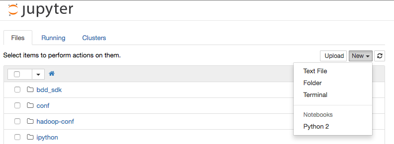
Go to http://localhost:18888 in your web browser, and from the New menu select a Python 2 notebook:
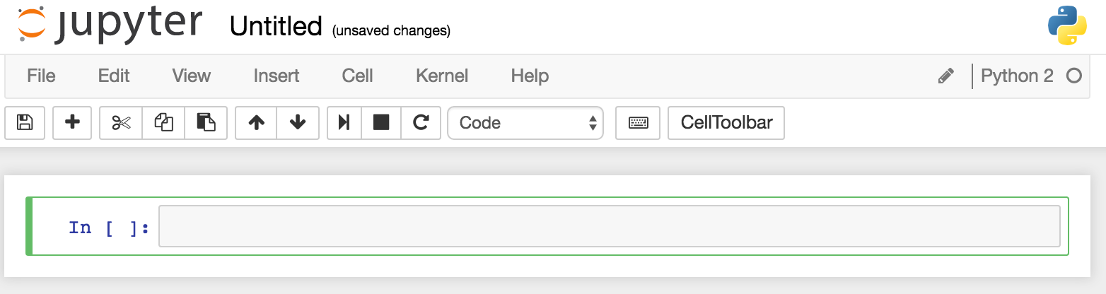
You should then see an empty notebook, ready for use:
The 'cell' (grey box after the In [ ]:) is where you enter code to run - type in execfile('ipython/00-bdd-shell-init.py') and press shift-Enter. This will execute it - if you don't press shift you just get a newline. Whilst it's executing you'll notice the line prefix changes from [ ] to [*], and in the terminal window from which you launched Jupyter you'll see some output related to the BDD Shell starting
WARNING: User-defined SPARK_HOME (/usr/lib/spark) overrides detected (/usr/lib/spark/).
WARNING: Running spark-class from user-defined location.
spark.driver.cores is set but does not apply in client mode.
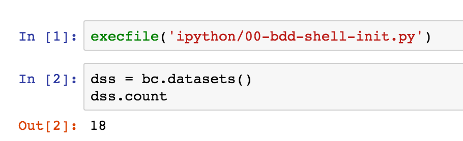
Now back in the Notebook, enter the following - use Enter, not Shift-enter, between lines:
dss = bc.datasets()
dss.count
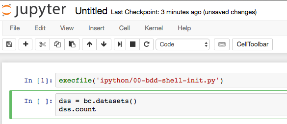
Now press shift-enter to execute it. This uses the pre-defined bc BDD context to get the datasets object, and return a count from it.
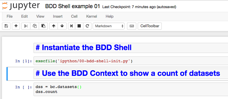
By clicking the + button on the toolbar, using the up and down arrows on the toolbar, and the Code/Markdown dropdown, it's possible to insert "cells" which are not code but instead commentary on what the code is. This way you can produce fully documented, but executable, code objects.
From the File menu give the notebook a name, and then Close and Halt, which destroys the Jupyter process ('kernel') that was executing the BDD Shell session. Back at the Jupyter main page, you'll note that a ipynb file has been created, which holds the notebook definition and can be downloaded, sent to colleagues, uploaded to blogs to share, saved in source control, and so on. Here's the file for the notebook above - note that it's hosted on gist, which automagically previews it as a Notebook, so click on Raw to see the actual code behind it.
The fantastically powerful thing about the Notebooks is that you can modify and re-run steps as you go -- but you never lose the history of how you got somewhere. Most people will be familar with learning or exploring a tool and its capabilities and eventually getting it to work - but no idea how they got there. Even for experienced users of a tool, being able to prove how to replicate a final result is important for (a) showing the evidence for how they got there and (b) enabling others to take that work and build on it.
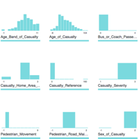
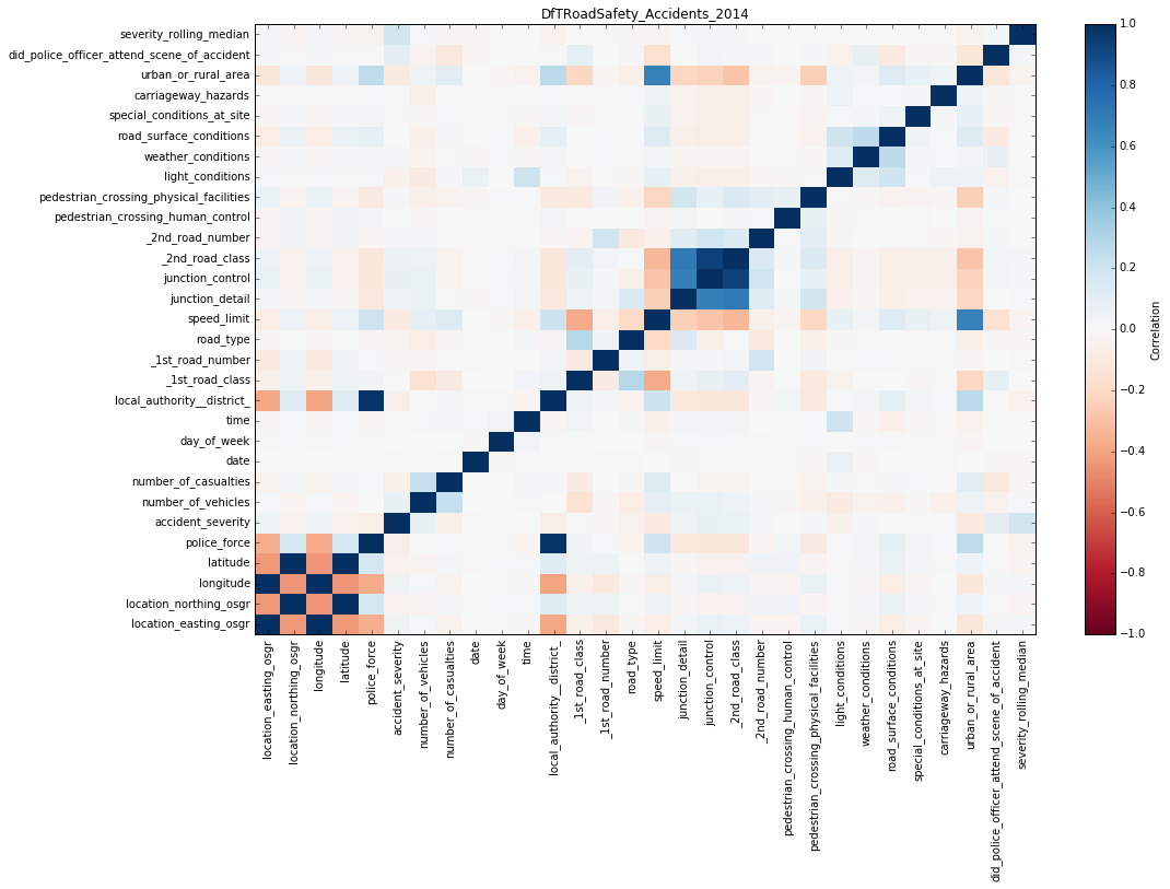
With an existing notebook file, whether a saved one you created or one that someone sent you, you can reopen it in Jupyter and re-execute it, in order to replicate the results previously seen. This is an important tenet of [data] science in general - show your workings, and it's great that Big Data Discovery supports this option. Obviously, showing the count of datasets is not so interesting or important to replicate. The real point here is being able to take datasets that you've got in BDD, done some joining and wrangling on already taking advantage of the GUI, and then dive deep into the data science and analytics world of things like Spark MLLib, Pandas, and so on. As a simple example, I can use a couple of python libraries (installed by default with Anaconda) to plot a correlation matrix for one of my BDD datasets:
As well as producing visualisations or calculations within BDD shell, the real power comes in being able to push the modified data back into Hive, and thus continue to work with it within BDD.
With Jupyter Notebooks not only can you share the raw notebooks for someone else to execute, you can export the results to HTML, PDF, and so on. Here's the notebook I started above, developed out further and exported to HTML - note how you can see not only the results, but exactly the code that I ran in order to get them. In this I took the dataset from BDD, added a column into it using a pandas windowing function, and then saved it back to a new Hive table:
(you can view the page natively here, and the ipynb here)
https://gist.github.com/rmoff/f1024dd043565cb8a58a0c54e9a782f2
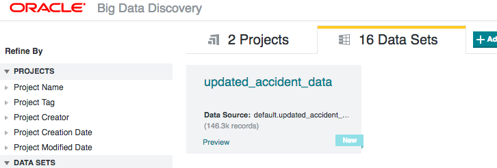
Once the data's been written back to Hive from the Python processing, I ran BDD's data_processing_CLI to add the new table back into BDD
/u01/bdd/v1.2.0/BDD-1.2.0.31.813/dataprocessing/edp_cli/data_processing_CLI --table updated_accident_data
And once that's run, I can then continue working with the data in BDD:
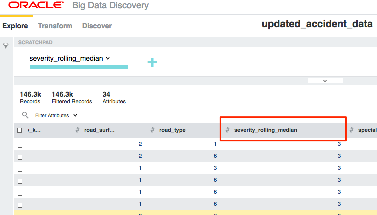
This workflow enables a continual loop of data wrangling, enrichment, advanced processing, and visualisation - all using the most appropriate tools for the job.
You can also use BDD Shell/Jupyter as another route for loading data into BDD. Whilst you can import CSV and XLS files into BDD directly through the web GUI, there are limitations - such as an XLS workbook with multiple sheets has to be imported one sheet at a time. I had a XLS file with over 40 sheets of reference data in it, which was not going to be time-efficient to load one at a time into BDD.
Pandas supports a lot of different input types - including Excel files. So by using Pandas to pull the data in, then convert it to a Spark dataframe I can write it to Hive, from where it can be imported to BDD. As before, the beauty of the Notebook approach is that I could develop and refine the code, and then simply share the Notebook here
https://gist.github.com/rmoff/3fa5d857df8ca5895356c22e420f3b22