Using R with Jupyter Notebooks and Oracle Big Data Discovery

Oracle's Big Data Discovery encompasses a good amount of exploration, transformation, and visualisation capabilities for datasets residing in your organisation’s data reservoir. Even with this though, there may come a time when your data scientists want to unleash their R magic on those same datasets. Perhaps the data domain expert has used BDD to enrich and cleanse the data, and now it's ready for some statistical analysis? Maybe you'd like to use R's excellent forecast package to predict the next six months of a KPI from the BDD dataset? And not only predict it, but write it back into the dataset for subsequent use in BDD? This is possible using BDD Shell and rpy2. It enables advanced analysis and manipulation of datasets already in BDD. These modified datasets can then be pushed back into Hive and then BDD.
BDD Shell provides a native Python environment, and you may opt to use the pandas library to work with BDD datasets as detailed here. In other cases you may simply prefer working with R, or have a particular library in mind that only R offers natively. In this article we’ll see how to do that. The "secret sauce" is rpy2 which enables the native use of R code within a python-kernel Jupyter Notebook.
As with previous articles I’m using a Jupyter Notebook as my environment. I’ll walk through the code here, and finish with a copy of the notebook so you can see the full process.
First we'll see how you can use R in Jupyter Notebooks running a python kernel, and then expand out to integrate with BDD too. You can view and download the first notebook here.
Import the RPY2 environment so that we can call R from Jupyter
import readline is necessary to workaround the error: /u01/anaconda2/lib/libreadline.so.6: undefined symbol: PC
import readline%load_ext rpy2.ipythonExample usage
Single inline command, prefixed with %R
%R X=c(1,4,5,7); sd(X); mean(X)array([ 4.25])
R code block, marked by %%R
%%R
Y = c(2,4,3,9)
summary(lm(Y~X))
Call:
lm(formula = Y ~ X)
Residuals:
1 2 3 4
0.88 -0.24 -2.28 1.64
Coefficients:
Estimate Std. Error t value Pr(>|t|)
(Intercept) 0.0800 2.3000 0.035 0.975
X 1.0400 0.4822 2.157 0.164
Residual standard error: 2.088 on 2 degrees of freedom
Multiple R-squared: 0.6993, Adjusted R-squared: 0.549
F-statistic: 4.651 on 1 and 2 DF, p-value: 0.1638
Graphics plot, output to the notebook
%R plot(X, Y)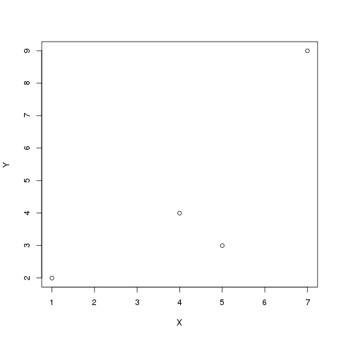
Pass Python variable to R using -i
import numpy as np
Z = np.array([1,4,5,10])
%R -i Z mean(Z)array([ 5.])
For more information see the documentation
Working with BDD Datasets from R in Jupyter Notebooks
Now that we've seen calling R in Jupyter Notebooks, let's see how to use it with BDD in order to access datasets. The first step is to instantiate the BDD Shell so that you can access the datasets in BDD, and then to set up the R environment using rpy2
execfile('ipython/00-bdd-shell-init.py')
%load_ext rpy2.ipython
I also found that I had to make readline available otherwise I got an error (/u01/anaconda2/lib/libreadline.so.6: undefined symbol: PC)
import readline
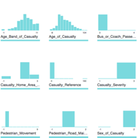
After this, we can import a BDD dataset, convert it to a Spark dataframe and then a pandas dataframe, ready for passing to R
ds = dss.dataset('edp_cli_edp_8d6fd230-8e99-449c-9480-0c2bddc4f6dc')
spark_df = ds.to_spark()
import pandas as pd
pandas_df = spark_df.toPandas()
Note that there is a lot of passing of the same dataframe into different memory structures here - from BDD dataset context to Spark to Pandas, and that’s before we’ve even hit R. It’s fine for ad-hoc wrangling but might start to be painful with very large datasets.
Now we use the rpy2 integration with Jupyter Notebooks and invoke R parsing of the cell’s contents, using the %%R syntax. Optionally, we can pass across variables with the -i parameter, which we’re doing here. Then we assign the dataframe to an R-notation variable (optional, but stylistically nice to do), and then use R's summary function to show a summary of each attribute:
%%R -i pandas_df
R.df <- pandas_df
summary(R.df)
vendorid     tpep_pickup_datetime tpep_dropoff_datetime passenger_count
 Min.   :1.000   Min.   :1.420e+12    Min.   :1.420e+12     Min.   :0.000
 1st Qu.:1.000   1st Qu.:1.427e+12    1st Qu.:1.427e+12     1st Qu.:1.000
 Median :2.000   Median :1.435e+12    Median :1.435e+12     Median :1.000
 Mean   :1.525   Mean   :1.435e+12    Mean   :1.435e+12     Mean   :1.679
 3rd Qu.:2.000   3rd Qu.:1.443e+12    3rd Qu.:1.443e+12     3rd Qu.:2.000
 Max.   :2.000   Max.   :1.452e+12    Max.   :1.452e+12     Max.   :9.000
 NA's   :12      NA's   :12           NA's   :12            NA's   :12
 trip_distance      pickup_longitude  pickup_latitude    ratecodeid
 Min.   :    0.00   Min.   :-121.93   Min.   :-58.43   Min.   : 1.000
 1st Qu.:    1.00   1st Qu.: -73.99   1st Qu.: 40.74   1st Qu.: 1.000
 Median :    1.71   Median : -73.98   Median : 40.75   Median : 1.000
 Mean   :    3.04   Mean   : -72.80   Mean   : 40.10   Mean   : 1.041
 3rd Qu.:    3.20   3rd Qu.: -73.97   3rd Qu.: 40.77   3rd Qu.: 1.000
 Max.   :67468.40   Max.   : 133.82   Max.   : 62.77   Max.   :99.000
 NA's   :12         NA's   :12        NA's   :12       NA's   :12
 store_and_fwd_flag dropoff_longitude dropoff_latitude  payment_type
 N   :992336        Min.   :-121.93   Min.   : 0.00    Min.   :1.00
 None:    12        1st Qu.: -73.99   1st Qu.:40.73    1st Qu.:1.00
 Y   :  8218        Median : -73.98   Median :40.75    Median :1.00
                    Mean   : -72.85   Mean   :40.13    Mean   :1.38
                    3rd Qu.: -73.96   3rd Qu.:40.77    3rd Qu.:2.00
                    Max.   :   0.00   Max.   :44.56    Max.   :5.00
                    NA's   :12        NA's   :12       NA's   :12
  fare_amount          extra            mta_tax          tip_amount
 Min.   :-170.00   Min.   :-1.0000   Min.   :-1.7000   Min.   :  0.000
 1st Qu.:   6.50   1st Qu.: 0.0000   1st Qu.: 0.5000   1st Qu.:  0.000
 Median :   9.50   Median : 0.0000   Median : 0.5000   Median :  1.160
 Mean   :  12.89   Mean   : 0.3141   Mean   : 0.4977   Mean   :  1.699
 3rd Qu.:  14.50   3rd Qu.: 0.5000   3rd Qu.: 0.5000   3rd Qu.:  2.300
 Max.   : 750.00   Max.   :49.6000   Max.   :52.7500   Max.   :360.000
 NA's   :12        NA's   :12        NA's   :12        NA's   :12
  tolls_amount      improvement_surcharge  total_amount       PRIMARY_KEY
 Min.   : -5.5400   Min.   :-0.3000       Min.   :-170.80   0-0-0   :      1
 1st Qu.:  0.0000   1st Qu.: 0.3000       1st Qu.:   8.75   0-0-1   :      1
 Median :  0.0000   Median : 0.3000       Median :  11.80   0-0-10  :      1
 Mean   :  0.3072   Mean   : 0.2983       Mean   :  16.01   0-0-100 :      1
 3rd Qu.:  0.0000   3rd Qu.: 0.3000       3rd Qu.:  17.80   0-0-1000:      1
 Max.   :503.0500   Max.   : 0.3000       Max.   : 760.05   0-0-1001:      1
 NA's   :12         NA's   :12            NA's   :12        (Other) :1000560
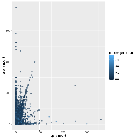
We can use native R code and R libraries including the excellent dplyr to lightly wrangle and then chart the data:
%%R

library(dplyr)
library(ggplot2)

R.df %>%
    filter(fare_amount > 0) %>%
    ggplot(aes(y=fare_amount, x=tip_amount,color=passenger_count)) +
    geom_point(alpha=0.5 )
Finally, using the -o flag on the %%R invocation, we can pass back variables from the R context back to pandas :
%%R -o R_output
R_output <-
    R.df %>%
    mutate(foo = 'bar')
and from there back to Spark and write the results to Hive:
spark_df2 = sqlContext.createDataFrame(R_output)
spark_df2.write.mode('Overwrite').saveAsTable('default.updated_dataset')
and finally ingest the new Hive table to BDD:
from subprocess import call
call(["/u01/bdd/v1.2.0/BDD-1.2.0.31.813/dataprocessing/edp_cli/data_processing_CLI","--table default.updated_dataset"])
You can download the notebook here.