I don't trust statistics and personally believe that at least 74% of them are wrong.... but I bet nearly 100% of people with any interest in fantasy (or just any) TV shows are watching the 7th series of Game of Thrones (GoT) by HBO.
If you are one of those, join me in the analysis of the latest tweets regarding the subject. Please be also aware that, if you're not on the latest episode, some spoilers may be revealed by this article. My suggestion is then to go back and watch the episodes first and then come back here for the analysis!

If you aren't part of the above group then ¯\_(ツ)_/¯. Still this post contains a lot of details on how to perform analysis on any tweet with Tableau and BigQuery together with Kafka sources and sink configurations. I'll leave to you to find another topic to put all this in practice.

Overall Setup

As described in my previous post on analysing Wimbledon tweets I've used Kafka for the tweet extraction phase. In this case however, instead of querying the data directly in Kafka with Presto, I'm landing the data into a Google BigQuery Table. The last step is optional, since as in last blog I was directly querying Kafka, but in my opinion represents the perfect use case of all technologies: Kafka for streaming and BigQuery for storing and querying data.
The endpoint is represented by Tableau, which has a native connector to BigQuery. The following image represents the complete flow

One thing to notice: at this point in time I'm using a on-premises installation of Kafka which I kept from my previous blog. However since source and target are natively cloud application I could easily move also Kafka in the cloud using for example the recently announced Confluent Kafka Cloud.

Now let's add some details about the overall setup.

Kafka

For the purpose of this blog post I've switched from the original Apache Kafka distribution to the open source Confluent Platform one. I've chosen the Confluent distribution for several reasons - it’s easier to install (e.g. with Docker images, yum, etc), it includes important components such as a Schema Registry - and it ships with several very useful connectors for Kafka Connect.

Kafka Connect is part of Apache Kafka, and provides a framework for easily ingesting streams of data into Kafka, and from Kafka out to target systems.

With this framework anybody can write a connector to streampush data from any system (Source Connector) to Kafka or streampull data from it to a target (Sink Connector). Moreover Kafka Connect provides the benefit of optionally converting the message body into Avro format which makes it easier to access and faster to retrieve. The schema for the Avro message is stored in the open-source Schema Registry, which is part of the Confluent Platform (or standalone, if you want). This is a list of available connectors developed and maintained either from Confluent or from the community. In this article I’m going to use two community connectors -- Twitter as the source and BigQuery as the sink.

Kafka Source for Twitter

In order to source from Twitter I've been using this connector. The setup is pretty easy: copy the source folder named kafka-connect-twitter-master under $CONFLUENT_HOME/share/java and modify the file TwitterSourceConnector.properties located under the config subfolder in order to include the connection details and the topics.

The configuration file in my case looked like the following:

name=connector1
tasks.max=1
connector.class=com.github.jcustenborder.kafka.connect.twitter.TwitterSourceConnector

# Set these required values
twitter.oauth.accessTokenSecret=<TWITTER_TOKEN_SECRET>
process.deletes=false
filter.keywords=#got,gameofthrones,stark,lannister,targaryen
kafka.status.topic=rm.got
kafka.delete.topic=rm.got
twitter.oauth.consumerSecret=<TWITTER_CONSUMER_SECRET>
twitter.oauth.accessToken=<TWITTER_ACCESS_TOKEN>
twitter.oauth.consumerKey=<TWITTER_CONSUMER_KEY>

Few things to notice:

• process.deletes=false: I'll not delete any message from the stream
• kafka.status.topic=rm.got: I'll write against a topic named rm.got
• filter.keywords=#got,gameofthrones,stark,lannister,targaryen: I'll take all the tweets with one of the following keywords included. The list could be expanded, this was just a test case.

All the work is done! the next step is to start the Kafka Connect execution via the following call from $CONFLUENT_HOME/share/java/kafka-connect-twitter

$CONFLUENT_HOME/bin/connect-standalone config/connect-avro-docker.properties config/TwitterSourceConnector.properties

I can see the flow of messages in Kafka using the avro-console-consumer command

./bin/kafka-avro-console-consumer --bootstrap-server localhost:9092 --property schema.registry.url=http://localhost:8081 --property print.key=true --topic twitter --from-beginning

You can see (or maybe it's a little bit difficult from the GIF) that the message body was transformed from JSON to AVRO format, the following is an example

{"CreatedAt":{"long":1502444851000},
"Id":{"long":895944759549640704},
"Text":{"string":"RT @haranatom: Daenerys Targaryen\uD83D\uDE0D https://t.co/EGQRvLEPIM"},
[...]
,"WithheldInCountries":[]}

Kafka Sink to BigQuery

Once the data is in Kafka, the next step is push it to the selected datastore: BigQuery. I can rely on Kafka Connect also for this task, with the related code written and supported by the community and available in github.

All I had to do is to download the code and change the file kcbq-connector/quickstart/properties/connector.properties

...
topics=rm.got
..
autoCreateTables=true
autoUpdateSchemas=true
...
# The name of the BigQuery project to write to
project=<NAME_OF_THE_BIGQUERY_PROJECT>
# The name of the BigQuery dataset to write to (leave the '.*=' at the beginning, enter your
# dataset after it)
datasets=.*=<NAME_OF_THE_BIGQUERY_DATASET>
# The location of a BigQuery service account JSON key file
keyfile=/home/oracle/Big-Query-Key.json

The changes included:

• the topic name to source from Kafka
• the project, dataset and Keyfile which are the connection parameters to BigQuery. Note that the Keyfile is automatically generated when creating a BigQuery service.

After verifying the settings, as per Kafka connect instructions, I had to create the tarball of the connector and extract it's contents

cd /path/to/kafka-connect-bigquery/
./gradlew clean confluentTarBall
mkdir bin/jar/ && tar -C bin/jar/ -xf bin/tar/kcbq-connector-*-confluent-dist.tar

The last step is to launch the connector by moving into the kcbq-connector/quickstart/ subfolder and executing

./connector.sh

Note that you may need to specify the CONFLUENT_DIR if the Confluent installation home is not in a sibling directory

export CONFLUENT_DIR=/path/to/confluent

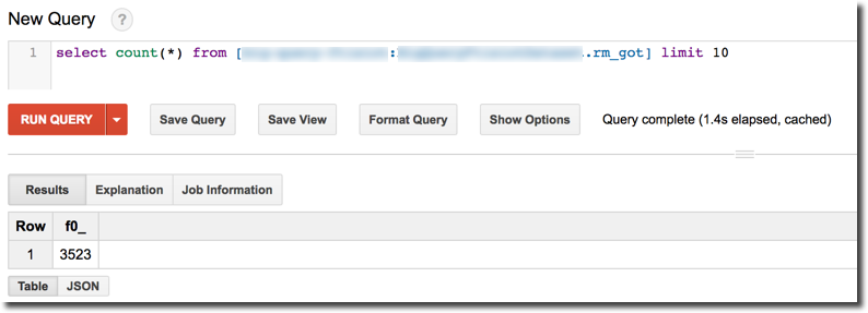
When everything start up without any error a table named rm_got (the name is automatically generated) appears in the BigQuery dataset I defined previously and starts populating.

A side note: I encountered a Java Heap Space error during the run of the BigQuery sink. This was resolved by increasing the heap space setting of the connector via the following call

export KAFKA_HEAP_OPTS="-Xms512m -Xmx1g"

BigQuery

BigQuery, based on Dremel's paper, is Google's proposition for an enterprise cloud datawarehouse which combines speed and scalability with separate pricing for storage and compute. If the cost of storage is common knowledge in the IT world, the compute cost is a fairly new concept. What this means is that the cost of the same query can vary depending on how the data is organized. In Oracle terms, we are used to associating the query cost to the one defined in the explain plan. In BigQuery that concept is translated from "performance cost" to also "financial cost" of a query: the more data a single query has to scan, the higher is the cost for it. This makes the work of optimizing data structures not only visible performance wise but also on the financial side.

For the purpose of the blog post, I had almost 0 settings to configure other than creating a Google Cloud Platform, creating a BigQuery project and a dataset.

During the Project creation phase, a Keyfile is generated and stored locally on the computer. This file contains all the credentials needed to connect to BigQuery from any external application, my suggestion is to store it in a secure place.

{
  "type": "service_account",
  "project_id": "<PROJECT_ID>",
  "private_key_id": "<PROJECT_KEY_ID>",
  "private_key": "<PRIVATE_KEY>",
  "client_email": "<E-MAIL>",
  "client_id": "<ID>",
  "auth_uri": "https://accounts.google.com/o/oauth2/auth",
  "token_uri": "https://accounts.google.com/o/oauth2/token",
  "auth_provider_x509_cert_url": "https://www.googleapis.com/oauth2/v1/certs",
  "client_x509_cert_url": "<URL>"
}

This file is used in the Kafka sink as we saw above.

Tableau

Once the data is landed in BigQuery, It's time to analyse it with Tableau!
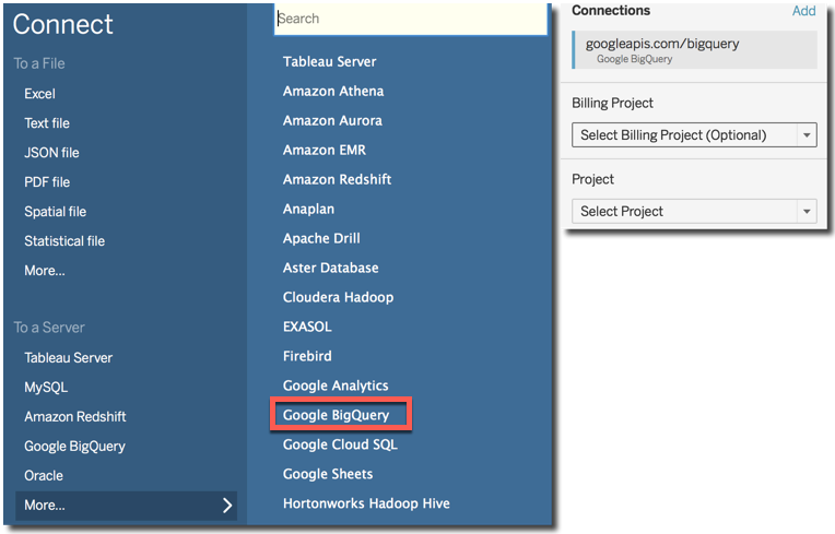
The Connection is really simple: from Tableau home I just need to select Connect-> To a Server -> Google BigQuery, fill in the connection details and select the project and datasource.

An important feature to set is the Use Legacy SQL checkbox in the datasource definition. Without this setting checked I wasn't able to properly query the BigQuery datasource. This is due to the fact that "Standard SQL" doesn't support nested columns while Legacy SQL (also known as BigQuery SQL) does, for more info check the related tableau website.

Analysing the data

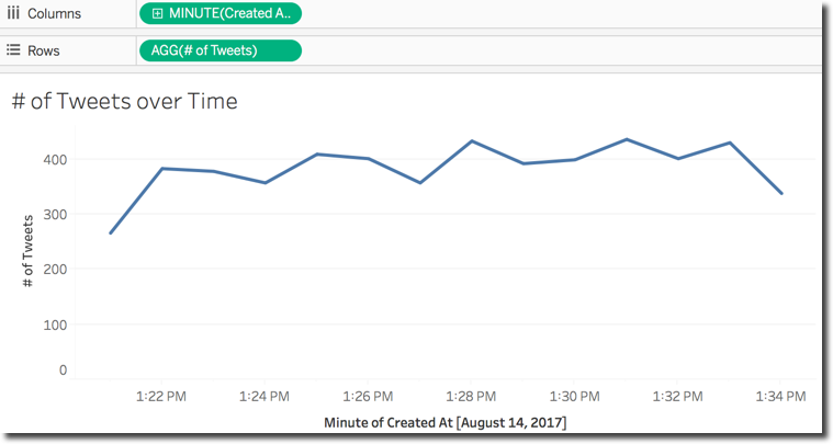
Now it starts the fun part: analysing the data! The integration between Tableau and BigQuery automatically exposes all the columns of the selected tables together with the correctly mapped datatypes, so I can immediately start playing with the dataset without having to worry about datatype conversions or date formats. I can simply include in the analysis the CreatedAt date and the Number of Records measure (named # of Tweets) and display the number of tweets over time.

Now I want to analyse where the tweets are coming from. I can use using the the Place.Country or the Geolocation.Latitude and Geolocation.Longitude fields in the tweet detail. Latitute and Longitude are more detailed while the Country is rolled up at state level, but both solutions have the same problem: they are available only for tweets with geolocation activated.

After adding Place.Country and # of Tweets in the canvas, I can then select the map as visualization. Two columns Latitude (generated) and Longitude (generated) are created on the fly mapping the country locations and the selected visualization is shown.

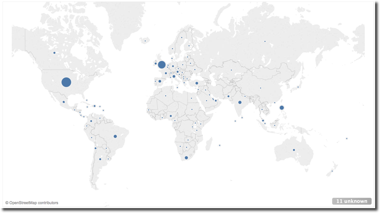
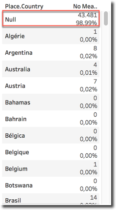
However as mentioned before, this map shows only a subset of the tweets since the majority of tweets (almost 99%) has no location.

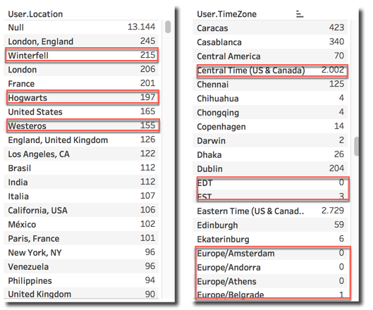
The fields User.Location and User.TimeZone suffer from a different problem: either are null or the possible values are not coming from a predefined list but are left to the creativity of the account owner which can type whatever string. As you can see, it seems we have some tweets coming from directly from Winterfell, Westeros, and interesting enough... Hogwarts!

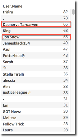
Checking the most engaged accounts based on User.Name field clearly shows that Daenerys and Jon Snow take the time to tweet between fighting Cercei and the Whitewalkers.

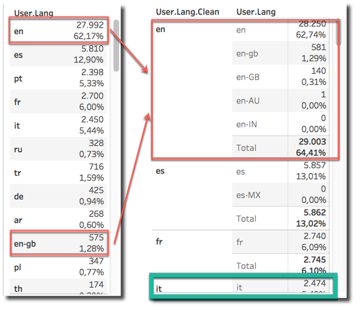
The field User.Lang can be used to identify the language of the User. However, when analysing the raw data, it can be noticed that there are language splits for regional language settings (note en vs en-gb). We can solve the problem by creating a new field User.Lang.Clean taking only the first part of the string with a formula like

IF  FIND([User.Lang],'-') =0
    THEN [User.Lang] 
    ELSE 
        LEFT([User.Lang],FIND([User.Lang],'-')-1)
END

With the interesting result of Italian being the 4th most used language, overtaking portuguese, and showing the high interest in the show in my home country.

Character and House Analysis

Still with me? So far we've done some pretty basic analysis on top of pre-built fields or with little transformations... now it's time to go deep into the tweet's Text field and check what the people are talking about!

The first thing I wanted to do is check mentions about the characters and related houses. The more a house is mentioned, the more should be relevant correct?
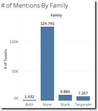
The first text analysis I want to perform was Stark vs Targaryen mention war: showing how many tweets were mentioning both, only one or none of two of the main houses. I achieved it with the below IF statement

IF contains(upper([Text]), 'STARK') AND contains(upper([Text]),'TARGARYEN')    
 THEN 'Both' 
 ELSEIF contains(upper([Text]), 'STARK') 
  THEN 'Stark' 
 ELSEIF contains(upper([Text]), 'TARGARYEN') 
  THEN 'Targaryen' 
 ELSE 'None' 
END

With the results supporting the house Stark

I can do the same at single character level counting the mentions on separate columns like for Jon Snow

IIF(contains(upper([Text]), 'JON') 
OR contains(upper([Text]),'SNOW'), 1,0)

Note the OR condition since I want to count as mentions both the words JON and SNOW since those can uniquely be referred at the same character. Similarly I can create a column counting the mentions to Arya Stark with the following formula

IIF(contains(upper([Text]), 'ARYA'), 1,0)

Note in this case I'm filtering only the name (ARYA) since Stark can be a reference to multiple characters (Sansa, Bran ...). I created several columns like the two above for some characters and displayed them in a histogram ordered by # of Mentions in descending order.

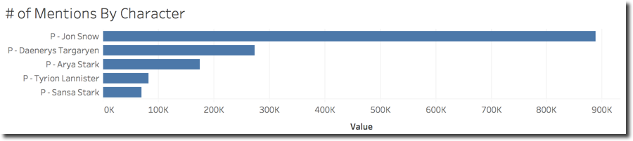
As expected, after looking at the Houses results above, Jon Snow is leading the user mentions with a big margin over the others with Daenerys in second place.

The methods mentioned above however have some big limitations:

• I need to create a different column for every character/house I want to analyse
• The formula complexity increases if I want to analyse more houses/characters at the same time

My goal would be to have an Excel file, where I set the research Key (like JON and SNOW) together with the related character and house and mash this data with the BigQuery table.

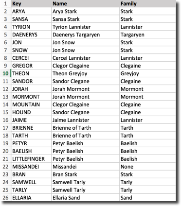
The joining key would be like

CONTAINS([BigQuery].[Text], [Excel].[Key]) >0

Unfortunately Tableau allows only = operators in text joining conditions during data blending making the above syntax impossible to implement. I have now three options:

• Give Up: Never if there is still hope!
• Move the Excel into a BigQuery table and resolve the problem there by writing a view on top of the data: works but increases the complexity on BigQuery side, plus most Tableau users will not have write access to related datasources.
• Find an alternative way of joining the data: If the CONTAINS join is not possible during data-blending phase, I may use it a little bit later...

Warning: the method mentioned below is not the optimal performance wise and should be used carefully since it causes data duplication if not handled properly.

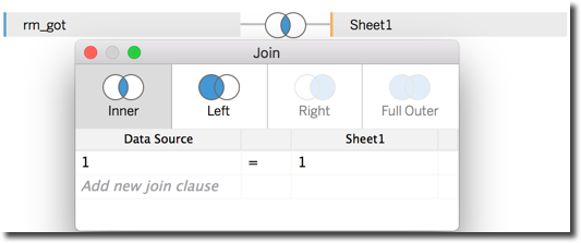
Without the option of using the CONTAINS I had to create a cartesian join during data-blending phase. By using a cartesian join every row in the BigQuery table is repeated for every row in the Excel table. I managed to create a cartesian join by simply put a 1-1 condition in the data-blending section.

I can then apply a filter on the resulting dataset to keep only the BigQuery rows mentioning one (or more) Key from the Excel file with the following formula.

IIF(CONTAINS(UPPER([Text]),[Key]),[Id],NULL)

This formula filters the tweet Id where the Excel's [Key] field is contained in the UPPER([Text]) coming from Twitter. Since there are multiple Keys assigned to the same character/house (see Jon Snow with both keywords JON and SNOW) the aggregation for this column is count distinct which in Tableau is achieved with COUNTD formula.
I can now simply drag the Name from the Excel file and the # of Mentions column with the above formula and aggregation method as count distinct.

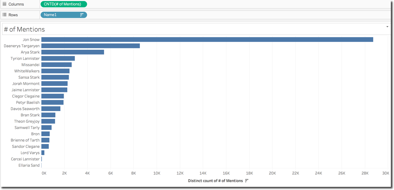
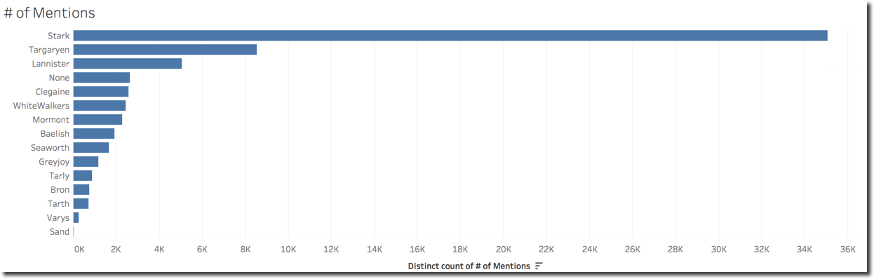
The beauty of this solution is that now if I need to do the same graph by house, I don't need to create columns with new formulas, but simply remove the Name field and replace it with Family coming from the Excel file.

Also if I forgot a character or family I simply need to add the relevant rows in the Excel lookup file and reload it, nothing to change in the formulas.

Sentiment Analysis

Another goal I had in mind when analysing GoT data was the sentiment analysis of tweets and the average sentiment associated to a character or house. Doing sentiment analysis in Tableau is not too hard, since we can reuse already existing packages coming from R.

For the Tableau-R integration to work I had to install and execute the RServe package from a workstation where R was already installed and set the connection in Tableau. More details on this configuration can be found in Tableau documentation

Once configured Tableau to call R functions it's time to analyse the sentiment. I used Syuzhet package (previously downloaded) for this purpose. The Sentiment calculation is done by the following formula:

SCRIPT_INT(
"library(syuzhet); 
r<-(get_sentiment(.arg1,method = 'nrc'))", 
ATTR([Text]))

Where

• SCRIPT_INT: The method will return an integer score for each Tweet with positives sentiments having positives scores and negative sentiments negative scores
• get_sentiment(.arg1,method = 'nrc'): is the function used
• ATTR([Text]): the input parameter of the function which is the tweet text

At this point I can see the score associated to every tweet, and since that R package uses dictionaries, I limited my research to tweets in english language (filtering on the column User.Lang.Clean mentioned above by en).

The next step is to average the sentiment by character, seems an easy step but devil is in the details! Tableau takes the output of the SCRIPT_INT call to R as aggregated metric, thus not giving any visual options to re-aggregate! Plus the tweet Text field must be present in the layout for the sentiment to be calculated otherwise the metric results NULL.

Fortunately there are functions, and specifically window functions like WINDOW_AVG allowing a post aggregation based of a formula defining the start and end. The other cool fact is that window function work per partition of the data and the start and end of the window can be defined using the FIRST() and LAST() functions.

We can now create an aggregated version of our Sentiment column with the following formula

WINDOW_AVG(FLOAT([Sentiment]), FIRST(), LAST())

This column will be repeated with the same value for all rows within the same "partition", in this case the character Name.

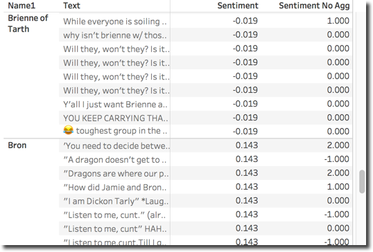
Be aware that this solution doesn't re-aggregate the data, we'll still see the data by single tweet Text and character Name. However the metric is calculated at total per character so graphs can be displayed.

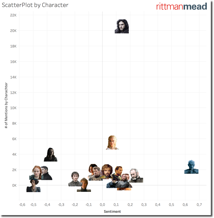
I wanted to show a Scatter Plot based on the # of Mentions and Sentiment of each character. With the window functions and the defined above it's as easy as dragging the fields in the proper place and select the scatter plot viz.

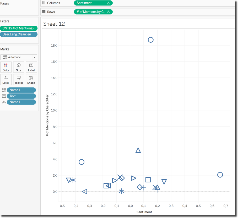
The default view is not very informative since I can't really associate a character to its position in the chart until I go over the related image. Fortunately Tableau allows the definition of custom shapes and I could easily assign character photos to related names.

If negative mentions for Littlefinger and Cercei was somehow expected, the characters with most negative sentiment are Sansa Stark, probably due to the mysterious letter found by Arya in Baelish room, and Ellaria Sand. On the opposite side we strangely see the Night King and more in general the WhiteWalkers with a very positive sentiment associated to them. Strange, this needs further investigation.

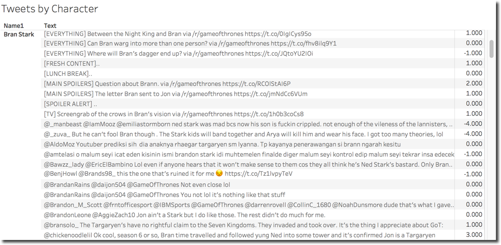
Deep Dive on Whitewalkers and Sansa

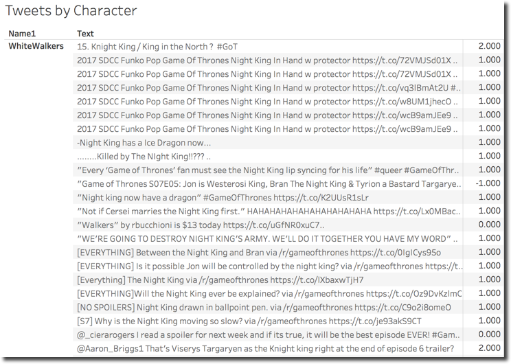
I can create a view per Character with associate tweets and sentiment score and filter it for the WhiteWalkers. Looks like there are great expectations for this character in the next episodes (the battle is coming) which are associated with positive sentiments.

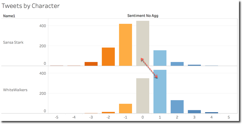
When analysing the detail of the number of tweets falling in each sentiment score category it's clear why Sansa and Whitewalkers have such a different sentiment average. Both appear as normal distributions, but the center of the Whitewalkers curve is around 1 (positive sentiment) while for Sansa is between -1 and 0 (negative sentiment).

This explanation however doesn't give me enough information, and want to understand more about what are the most used words included in tweets mentioning WhiteWalkers or Night King.

Warning: the method mentioned above is not the optimal performance wise and should be used carefully since it causes data duplication if not handled properly.

There is no easy way to do so directly in Tableau, even using R since all the functions expect the output size to be 1-1 with the input, like sentiment score and text.
For this purpose I created a view on top of the BigQuery table directly in Tableau using the New Custom SQL option. The SQL used is the following

SELECT  ID, REPLACE(REPLACE(SPLIT(UPPER(TEXT),' '),'#',''),'@','')  word FROM [Dataset.rm_got]

The SPLIT function divides the Text field in multiple rows one for every word separated by space. This is a very basic split and can of course be enhanced if needed. On top of it the SQL removes references to # and @. Since the view contains the tweet's Id field, this can be used to join this dataset with the main table.

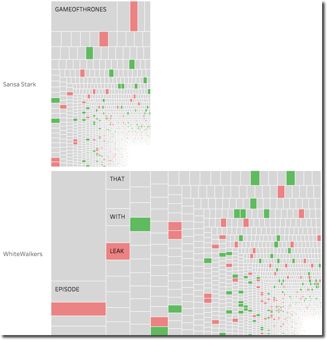
The graph showing the overall words belonging to characters is not really helpful since the amount of words (even if I included only the ones with more than e chars) is too huge to be analysed properly.

When analysing the single words in particular tweets I can clearly see that the Whitewalkers sentiment is driven by words like King, Iron, Throne having a positive sentiment. On the other hand Sansa stark is penalized by words like Kill and Fight probably due to the possible troubles with Arya.

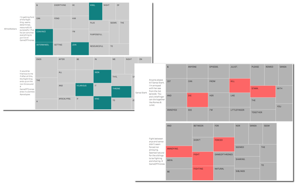
One thing to mention is that the word Stark is classified with a negative sentiment due to the general english dictionary used for the scoring. This affects all the tweets and in particular the average scores of all the characters belonging to the House Stark. A new "GoT" dictionary should be created and used in order to avoid those kind of misinterpretations.

Also when talking about "Game of Thrones", words like Kill or Death can have positive or negative meaning depending on the sentence, a imaginary tweet like

Finally Arya kills Cercei

Should have a positive sentiment for Arya and a negative for Cercei, but this is where automatic techniques of sentiment classification show their limits. Not even a new dictionary could help in this case.

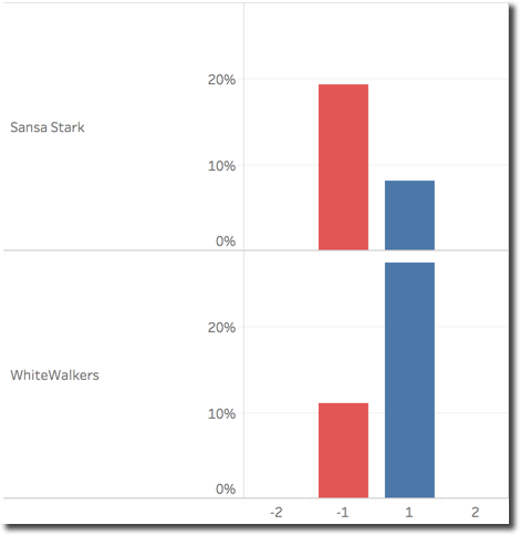
The chart below shows the percentage of words classified with positive (score 1 or 2) or negative (score -1 or -2) for the two selected characters. We can clearly see that Sansa has more negative words than positive as expected while Whitewalkers is on the opposite side.

Furthermore the overall sentiment for the two characters may be explained by the following graph. This shows for every sentence sentiment category (divided in bins Positive, Neutral, Negative), an histogram based on the count of words by single word sentiment. We can clearly see how words with positive sentiment are driving the Positive sentence category (and the opposite).

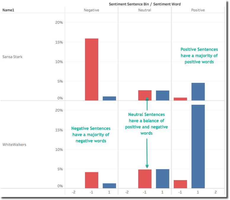
Finally the last graph shows the words that have mostly impacted the overall positive and negative sentiment for both characters.

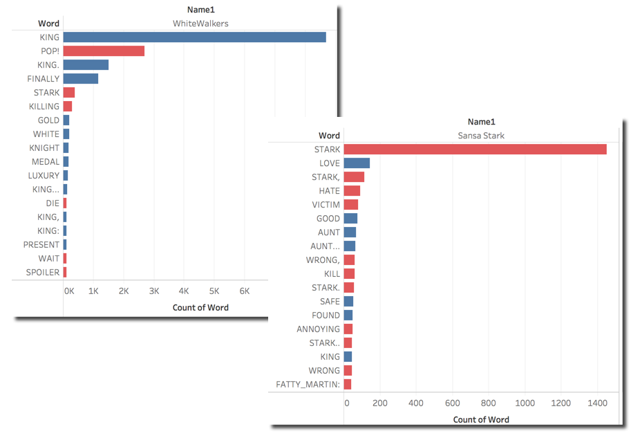
We can clearly see that Sansa negative sentiment is due to Stark, Hate and Victim. On the other side Whitewalkers positive sentiment is due to words like King (Night King is the character) and Finally probably due to the battle coming in the next episode. As you can see there are also multiple instances of the King word due to different punctualization preceeding or following the world. I stated above that the BigQuery SQL extracting the words via the SPLIT function was very basic, we can now see why. Little enhancements in the function would aggregate properly the words.

Are you still there? Do you wonder what's left? Well there is a whole set of analysis that can be done on top of this dataset, including checking the sentiment behaviour by time during the live event or comparing this week's dataset with the next episode's one. The latter may happen next week so... Keep in touch!

Hope you enjoyed the analysis... otherwise... Dracarys!