Taking KSQL for a Spin Using Real-time Device Data

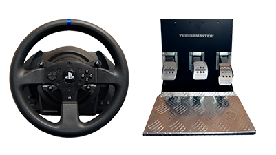
Evaluating KSQL has been high on my to-do list ever since it was released back in August. I wanted to experiment with it using an interesting, high velocity, real-time data stream that would allow me to analyse events at the millisecond level, rather than seconds or minutes. Finding such a data source, that is free of charge and not the de facto twitter stream, is tricky. So, after some pondering, I decided that I'd use my Thrustmaster T300RS Steering Wheel/Pedal Set gaming device as a data source,

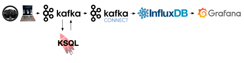
The idea being that the data would be fed into Kafka, processed in real-time using KSQL and visualised in Grafana.

This is the end to end pipeline that I created...

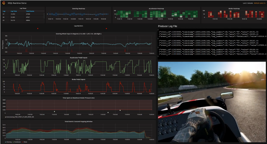
...and this is the resulting real-time dashboard running alongside a driving game and a log of the messages being sent by the device.

This article will explain how the above real-time dashboard was built using only KSQL...and a custom Kafka producer.

I'd like to point out, that although the device I'm using for testing is unconventional, when considered in the wider context of IoT's, autonomous driving, smart automotives or any device for that matter, it will be clear to see that the low latency, high throughput of Apache Kafka, coupled with Confluent's KSQL, can be a powerful combination.

I'd also like to point out, that this article is not about driving techniques, driving games or telemetry analysis. However, seeing as the data source I'm using is intrinsically tied to those subjects, the concepts will be discussed to add context. I hope you like motorsports!

Writing a Kafka Producer for a T300RS

The T300RS is attached to my Windows PC via a USB cable, so the first challenge was to try and figure out how I could get steering, braking and accelerator inputs pushed to Kafka. Unsurprisingly, a source connector for a "T300RS Steering Wheel and Pedal Set" was not listed on the Kafka Connect web page - a custom producer was the only option.

To access the data being generated by the T300RS, I had 2 options, I could either use an existing Telemetry API from one of my racing games, or I could access it directly using the Windows DirectX API. I didn't want to have to have a game running in the background in order to generate data, so I decided to go down the DirectX route. This way, the data is raw and available, with or without an actual game engine running.

The producer was written using the SharpDX .NET wrapper and Confluent's .NET Kafka Client. The SharpDX directinput API allows you to poll an attached input device (mouse, keyboard, game controllers etc.) and read its buffered data. The buffered data returned within each polling loop is serialized into JSON and sent to Kafka using the .NET Kafka Client library.

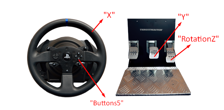
A single message is sent to a topic in Kafka called raw_axis_inputs every time the state of one the device's axes changes. The device has several axes, in this article I am only interested in the Wheel, Accelerator, Brake and the X button.

{  
    "event_id":4300415,         // Event ID unique over all axis state changes
    "timestamp":1508607521324,  // The time of the event
    "axis":"Y",                 // The axis this event belongs to
    "value":32873.0             // the current value of the axis
}

This is what a single message looks like. In the above message the Brake axis state was changed, i.e. it moved to a new position with value 32873.

You can see below which inputs map to the each reported axis from the device.

Here is a sample from the producer's log file.

{"event_id":4401454,"timestamp":1508687373018,"axis":"X","value":33007.0}
{"event_id":4401455,"timestamp":1508687373018,"axis":"RotationZ","value":62515.0}
{"event_id":4401456,"timestamp":1508687373018,"axis":"RotationZ","value":62451.0}
{"event_id":4401457,"timestamp":1508687373018,"axis":"X","value":33011.0}
{"event_id":4401458,"timestamp":1508687373018,"axis":"RotationZ","value":62323.0}
{"event_id":4401459,"timestamp":1508687373018,"axis":"RotationZ","value":62258.0}
{"event_id":4401460,"timestamp":1508687373034,"axis":"X","value":33014.0}
{"event_id":4401461,"timestamp":1508687373034,"axis":"X","value":33017.0}
{"event_id":4401462,"timestamp":1508687373065,"axis":"RotationZ","value":62387.0}
{"event_id":4401463,"timestamp":1508687373081,"axis":"RotationZ","value":62708.0}
{"event_id":4401464,"timestamp":1508687373081,"axis":"RotationZ","value":62901.0}
{"event_id":4401465,"timestamp":1508687373081,"axis":"RotationZ","value":62965.0}
{"event_id":4401466,"timestamp":1508687373097,"axis":"RotationZ","value":64507.0}
{"event_id":4401467,"timestamp":1508687373097,"axis":"RotationZ","value":64764.0}
{"event_id":4401468,"timestamp":1508687373097,"axis":"RotationZ","value":64828.0}
{"event_id":4401469,"timestamp":1508687373097,"axis":"RotationZ","value":65021.0}
{"event_id":4401470,"timestamp":1508687373112,"axis":"RotationZ","value":65535.0}
{"event_id":4401471,"timestamp":1508687373268,"axis":"X","value":33016.0}
{"event_id":4401472,"timestamp":1508687373378,"axis":"X","value":33014.0}
{"event_id":4401473,"timestamp":1508687377972,"axis":"Y","value":65407.0}
{"event_id":4401474,"timestamp":1508687377987,"axis":"Y","value":64057.0}
{"event_id":4401475,"timestamp":1508687377987,"axis":"Y","value":63286.0}

You can tell by looking at the timestamps, it's possible to have multiple events generated within the same millisecond, I was unable to get microsecond precision from the device unfortunately. When axes, "X", "Y" and "RotationZ" are being moved quickly at the same time (a bit like a child driving one of those coin operated car rides you find at the seaside) the device generates approximately 500 events per second.

Creating a Source Stream

Now that we have data streaming to Kafka from the device, it's time to fire up KSQL and start analysing it. The first thing we need to do is create a source stream. The saying "Every River Starts with a Single Drop" is quite fitting here, especially in the context of stream processing. The raw_axis_inputs topic is our "Single Drop" and we need to create a KSQL stream based on top of it.

CREATE STREAM raw_axis_inputs ( \
     event_id BIGINT, \
     timestamp BIGINT, \
     axis VARCHAR, \
     value DOUBLE ) \
 WITH (kafka_topic = 'raw_axis_inputs', value_format = 'JSON');

With the stream created we can we can now query it. I'm using the default auto.offset.reset = latest as I have the luxury of being able to blip the accelerator whenever I want to generate new data, a satisfying feeling indeed.

ksql> SELECT * FROM raw_axis_inputs;
1508693510267 | null | 4480290 | 1508693510263 | RotationZ | 65278.0
1508693510269 | null | 4480291 | 1508693510263 | RotationZ | 64893.0
1508693510271 | null | 4480292 | 1508693510263 | RotationZ | 63993.0
1508693510273 | null | 4480293 | 1508693510263 | RotationZ | 63094.0
1508693510275 | null | 4480294 | 1508693510279 | RotationZ | 61873.0
1508693510277 | null | 4480295 | 1508693510279 | RotationZ | 60716.0
1508693510279 | null | 4480296 | 1508693510279 | RotationZ | 60267.0

Derived Streams

We now have our source stream created and can start creating some derived streams from it. The first derived stream we are going to create filters out 1 event. When the X button is pressed it emits a value of 128, when it's released it emits a value of 0.

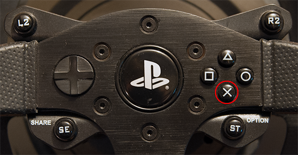
To simplify this input, I'm filtering out the release event. We'll see what the X button is used for later in the article.

CREATE STREAM axis_inputs WITH (kafka_topic = 'axis_inputs') AS \
SELECT  event_id, \
        timestamp, \
        axis, \
        value \
FROM    raw_axis_inputs \
WHERE   axis != 'Buttons5' OR value != 0.0;

From this stream we are going to create 3 further streams, one for the brake, one the accelerator and one for the wheel.

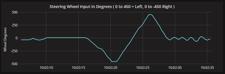
All 3 axes emit values in the range of 0-65535 across their full range. The wheel emits a value of 0 when rotated fully left, a value of 65535 when rotated fully right and 32767 when dead centre. The wheel itself is configured to rotate 900 degrees lock-to-lock, so it would be nice to report its last state change in degrees, rather than from a predetermined integer range. For this we can create a new stream, that includes only messages where the axis = 'X', and the axis values are translated into the range of -450 degrees to 450 degrees. With this new value translation, maximum rotation left now equates to 450 degrees and maximum rotation right equates -450 degrees, 0 is now dead centre.

CREATE STREAM steering_inputs WITH (kafka_topic = 'steering_inputs') AS \
  SELECT  axis, \
          event_id, \
          timestamp, \
          (value / (65535.0 / 900.0) - 900 / 2) * -1 as value \
  FROM    axis_inputs \
  WHERE   axis = 'X';

If we now query our new stream and move the wheel slowly around dead centre, we get the following results

ksql> select timestamp, value from steering_inputs;

1508711287451 | 0.6388888888889142
1508711287451 | 0.4305555555555429
1508711287451 | 0.36111111111108585
1508711287451 | 0.13888888888891415
1508711287451 | -0.0
1508711287467 | -0.041666666666685614
1508711287467 | -0.26388888888891415
1508711287467 | -0.3333333333333144
1508711287467 | -0.5277777777777715
1508711287467 | -0.5972222222222285

The same query while the wheel is rotated fully left

1508748345943 | 449.17601281757845
1508748345943 | 449.3270771343557
1508748345943 | 449.5330739299611
1508748345943 | 449.67040512703136
1508748345959 | 449.8214694438087
1508748345959 | 449.95880064087896
1508748345959 | 450.0

And finally, rotated fully right.

1508748312803 | -449.3408102540627
1508748312803 | -449.4369420920119
1508748312818 | -449.67040512703136
1508748312818 | -449.7390707255665
1508748312818 | -449.9725337605859
1508748312818 | -450.0

Here's the data plotted in Grafana.

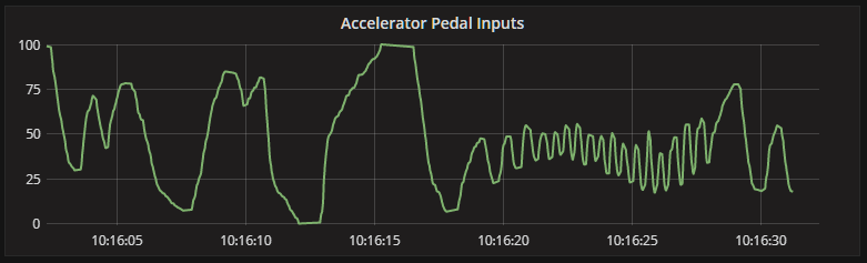
We now need to create 2 more derived streams to handle the accelerator and the brake pedals. This time, we want to translate the values to the range 0-100. When a pedal is fully depressed it should report a value of 100 and when fully released, a value of 0.

CREATE STREAM accelerator_inputs WITH (kafka_topic = 'accelerator_inputs') AS \
SELECT  axis, \
        event_id, \
        timestamp, \
        100 - (value / (65535.0 / 100.0)) as value \
FROM    axis_inputs \
WHERE   axis = 'RotationZ';

Querying the accelerator_inputs stream while fully depressing the accelerator pedal displays the following. (I've omitted many records in the middle to keep it short)

ksql> SELECT timestamp, value FROM accelerator_inputs;
1508749747115 | 0.0
1508749747162 | 0.14198473282442592
1508749747193 | 0.24122137404580712
1508749747209 | 0.43664122137404604
1508749747225 | 0.5343511450381726
1508749747287 | 0.6335877862595396
1508749747318 | 0.7312977099236662
1508749747318 | 0.8290076335877927
1508749747334 | 0.9267175572519051
1508749747381 | 1.0259541984732863
...
...
1508749753943 | 98.92519083969465
1508749753959 | 99.02290076335878
1508749753959 | 99.1206106870229
1508749753959 | 99.21832061068702
1508749753975 | 99.31603053435114
1508749753975 | 99.41374045801527
1508749753975 | 99.5114503816794
1508749753990 | 99.60916030534351
1508749753990 | 99.70687022900763
1508749753990 | 99.80458015267176
1508749754006 | 100.0

...and displayed in Grafana

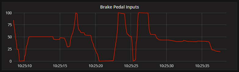
Finally, we create the brake stream, which has the same value translation as the accelerator stream, so I won't show the query results this time around.

CREATE STREAM brake_inputs WITH (kafka_topic = 'brake_inputs') AS \
SELECT  axis, \
        event_id, \
        timestamp, \
        100 - (value / (65535 / 100)) as value \
FROM    axis_inputs \
WHERE   axis = 'Y';	

Braking inputs in Grafana.

Smooth is Fast

It is a general rule of thumb in motorsports that "Smooth is Fast", the theory being that the less steering, accelerator and braking inputs you can make while still keeping the car on the desired racing line, results in a faster lap time. We can use KSQL to count the number of inputs for each axis over a Hopping Window to try and capture overall smoothness. To do this, we create our first KSQL table.

CREATE TABLE axis_events_hopping_5s_1s \
WITH (kafka_topic = 'axis_events_hopping_5s_1s') AS \
SELECT  axis, \
        COUNT(*) AS event_count \
FROM    axis_inputs \
WINDOW HOPPING (SIZE 5 SECOND, ADVANCE BY 1 SECOND) \
GROUP BY axis;

A KSQL table is basically a view over an existing stream or another table. When a table is created from a stream, it needs to contain an aggregate function and group by clause. It's these aggregates that make a table stateful, with the underpinning stream updating the table's current view in the background. If you create a table based on another table you do not need to specify an aggregate function or group by clause.

The table we created above specifies that data is aggregated over a Hopping Window. The size of the window is 5 seconds and it will advance or hop every 1 second. This means that at any one time, there will be 5 open windows, with new data being directed to each window based on the key and the record's timestamp.

You can see below when we query the stream, that we have 5 open windows per axis, with each window 1 second apart.

ksql> SELECT * FROM axis_events_hopping_5s_1s;
1508758267000 | X : Window{start=1508758267000 end=-} | X | 56
1508758268000 | X : Window{start=1508758268000 end=-} | X | 56
1508758269000 | X : Window{start=1508758269000 end=-} | X | 56
1508758270000 | X : Window{start=1508758270000 end=-} | X | 56
1508758271000 | X : Window{start=1508758271000 end=-} | X | 43
1508758267000 | Y : Window{start=1508758267000 end=-} | Y | 25
1508758268000 | Y : Window{start=1508758268000 end=-} | Y | 25
1508758269000 | Y : Window{start=1508758269000 end=-} | Y | 25
1508758270000 | Y : Window{start=1508758270000 end=-} | Y | 32
1508758271000 | Y : Window{start=1508758271000 end=-} | Y | 32
1508758267000 | RotationZ : Window{start=1508758267000 end=-} | RotationZ | 67
1508758268000 | RotationZ : Window{start=1508758268000 end=-} | RotationZ | 67
1508758269000 | RotationZ : Window{start=1508758269000 end=-} | RotationZ | 67
1508758270000 | RotationZ : Window{start=1508758270000 end=-} | RotationZ | 67
1508758271000 | RotationZ : Window{start=1508758271000 end=-} | RotationZ | 39

This data is going to be pushed into InfluxDB and therefore needs a timestamp column. We can create a new table for this, that includes all columns from our current table, plus the rowtime.

CREATE TABLE axis_events_hopping_5s_1s_ts \
WITH (kafka_topic = 'axis_events_hopping_5s_1s_ts') AS \
SELECT  rowtime AS timestamp, * \
FROM    axis_events_hopping_5s_1s;

And now, when we query this table we can see we have all the columns we need.

ksql> select timestamp, axis, event_count from axis_events_hopping_5s_1s_ts;
1508761027000 | RotationZ | 61
1508761028000 | RotationZ | 61
1508761029000 | RotationZ | 61
1508761030000 | RotationZ | 61
1508761031000 | RotationZ | 61
1508761028000 | Y | 47
1508761029000 | Y | 47
1508761030000 | Y | 47
1508761031000 | Y | 47
1508761032000 | Y | 47
1508761029000 | X | 106
1508761030000 | X | 106
1508761031000 | X | 106
1508761032000 | X | 106
1508761033000 | X | 106

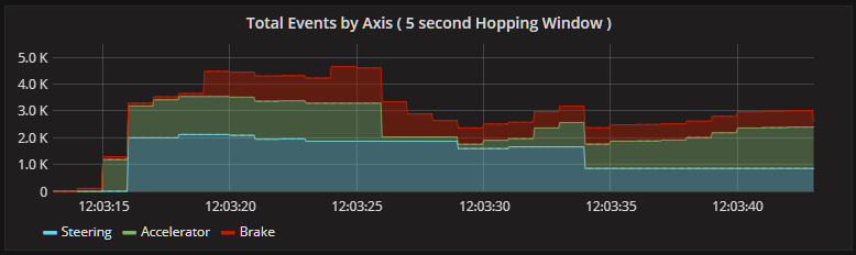
This is the resulting graph in Grafana with each axis stacked on top of each other giving a visual representation of the total number of events overall and total per axis. The idea here being that if you can drive a lap with less overall inputs or events then the lap time should be faster.

Calculating Lap Times

To calculate lap times, I needed a way of capturing the time difference between 2 separate events in a stream. Remember that the raw data is coming directly from the device and has no concept of lap, lap data is handled by a game engine.
I needed a way to inject an event into the stream when I crossed the start/finish line of any given race track. To achieve this, I modified the custom producer to increment a counter every time the X button was pressed and added a new field to the JSON message called lap_number.

I then needed to recreate my source stream and my initial derived stream to include this new field

New source stream

CREATE STREAM raw_axis_inputs ( \
     event_id BIGINT, \
     timestamp BIGINT, \
     lap_number BIGINT, \
     axis VARCHAR, \
     value DOUBLE ) \
 WITH (kafka_topic = 'raw_axis_inputs', value_format = 'JSON');

New derived stream.

CREATE STREAM axis_inputs WITH (kafka_topic = 'axis_inputs') AS \
SELECT  event_id, \
        timestamp, \
        lap_number, \
        axis, \
        value \
FROM    raw_axis_inputs \
WHERE   axis != 'Buttons5' OR value != 0.0;

Now when I query the axis_inputs stream and press the X button a few times we can see an incrementing lap number.

ksql> SELECT timestamp, lap_number, axis, value FROM axis_inputs;
1508762511506 | 6 | X | 32906.0
1508762511553 | 6 | X | 32907.0
1508762511803 | 6 | X | 32909.0
1508762512662 | 7 | Buttons5 | 128.0
1508762513178 | 7 | X | 32911.0
1508762513256 | 7 | X | 32913.0
1508762513318 | 7 | X | 32914.0
1508762513381 | 7 | X | 32916.0
1508762513459 | 7 | X | 32918.0
1508762513693 | 7 | X | 32919.0
1508762514584 | 8 | Buttons5 | 128.0
1508762515021 | 8 | X | 32921.0
1508762515100 | 8 | X | 32923.0
1508762515209 | 8 | X | 32925.0
1508762515318 | 8 | X | 32926.0
1508762515678 | 8 | X | 32928.0
1508762516756 | 8 | X | 32926.0
1508762517709 | 9 | Buttons5 | 128.0
1508762517756 | 9 | X | 32925.0
1508762520381 | 9 | X | 32923.0
1508762520709 | 9 | X | 32921.0
1508762520881 | 10 | Buttons5 | 128.0
1508762521396 | 10 | X | 32919.0
1508762521568 | 10 | X | 32918.0
1508762521693 | 10 | X | 32916.0
1508762521803 | 10 | X | 32914.0

The next step is to calculate the time difference between each "Buttons5" event (the X button). This required 2 new tables. The first table below captures the latest values using the MAX() function from the axis_inputs stream where the axis = 'Buttons5'

CREATE TABLE lap_marker_data WITH (kafka_topic = 'lap_marker_data') AS \
SELECT  axis, \
        MAX(event_id) AS lap_start_event_id, \
        MAX(timestamp) AS lap_start_timestamp, \ 
        MAX(lap_number) AS lap_number \
FROM    axis_inputs \
WHERE   axis = 'Buttons5' \
GROUP BY axis;

When we query this table, a new row is displayed every time the X button is pressed, reflecting the latest values from the stream.

ksql> SELECT axis, lap_start_event_id, lap_start_timestamp, lap_number FROM lap_marker_data;
Buttons5 | 4692691 | 1508763302396 | 15
Buttons5 | 4693352 | 1508763306271 | 16
Buttons5 | 4693819 | 1508763310037 | 17
Buttons5 | 4693825 | 1508763313865 | 18
Buttons5 | 4694397 | 1508763317209 | 19

What we can now do is join this table to a new stream.

CREATE STREAM lap_stats WITH (kafka_topic = 'lap_stats') AS \
SELECT  l.lap_number as lap_number, \
        l.lap_start_event_id, \
        l.lap_start_timestamp, \
        a.timestamp AS lap_end_timestamp, \
        (a.event_id - l.lap_start_event_id) AS lap_events, \
        (a.timestamp - l.lap_start_timestamp) AS laptime_ms \
FROM 	  axis_inputs a LEFT JOIN lap_marker_data l ON a.axis = l.axis \
WHERE   a.axis = 'Buttons5';	

 Message
----------------
Stream created

ksql> describe lap_stats;

 Field               | Type
---------------------------------------
 ROWTIME             | BIGINT
 ROWKEY              | VARCHAR (STRING)
 LAP_NUMBER          | BIGINT
 LAP_START_EVENT_ID  | BIGINT
 LAP_START_TIMESTAMP | BIGINT
 LAP_END_TIMESTAMP   | BIGINT
 LAP_EVENTS          | BIGINT
 LAPTIME_MS          | BIGINT

This new stream is again based on the axis_inputs stream where the axis = 'Buttons5'. We are joining it to our lap_marker_data table which results in a stream where every row includes the current and previous values at the point in time when the X button was pressed.

A quick query should illustrate this (I've manually added column heading to make it easier to read)

ksql> SELECT lap_number, lap_start_event_id, lap_start_timestamp, lap_end_timestamp, lap_events, laptime_ms FROM lap_stats;

LAP  START_EV  START_TS        END_TS          TOT_EV  LAP_TIME_MS
36 | 4708512 | 1508764549240 | 1508764553912 | 340   | 4672
37 | 4708852 | 1508764553912 | 1508764567521 | 1262  | 13609
38 | 4710114 | 1508764567521 | 1508764572162 | 1174  | 4641
39 | 4711288 | 1508764572162 | 1508764577865 | 1459  | 5703
40 | 4712747 | 1508764577865 | 1508764583725 | 939   | 5860
41 | 4713686 | 1508764583725 | 1508764593475 | 2192  | 9750
42 | 4715878 | 1508764593475 | 1508764602318 | 1928  | 8843

We can now see the time difference, in milliseconds ( LAP_TIME_MS ), between each press of the X button. This data can now be displayed in Grafana.

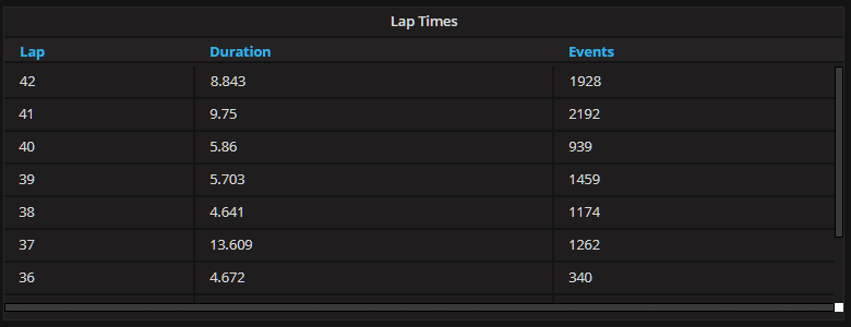
The data is also being displayed along the top of the dashboard, aligned above the other graphs, as a ticker to help visualize lap boundaries across all axes.

Anomaly Detection

A common use case when performing real-time stream analytics is Anomaly Detection, the act of detecting unexpected events, or outliers, in a stream of incoming data. Let's see what we can do with KSQL in this regard.

Driving Like a Lunatic?

As mentioned previously, Smooth is Fast, so it would be nice to be able to detect some form of erratic driving. When a car oversteers, the rear end of the car starts to rotate around a corner faster than you'd like, to counteract this motion, quick steering inputs are required to correct it. On a smooth lap you will only need a small part of the total range of the steering wheel to safely navigate all corners, when you start oversteering you will need make quick, but wider use of the total range of the wheel to keep the car on the track and prevent crashing.

To try and detect oversteer we need to create another KSQL table, this time based on the steering_inputs stream. This table counts steering events across a very short hopping window. Events are counted only if the rotation exceeds 180 degrees (sharp left rotation) or is less than -180 degrees (sharp right rotation)

CREATE TABLE oversteer WITH (kafka_topic = 'oversteer') AS \
SELECT  axis, \
        COUNT(*) \
FROM    steering_inputs \
WINDOW HOPPING (SIZE 100 MILLISECONDS, ADVANCE BY 10 MILLISECONDS) \
WHERE   value > 180 or value < -180 \
GROUP by axis;

We now create another table that includes the timestamp for InfluxDB.

CREATE TABLE oversteer_ts WITH (kafka_topic = 'oversteer_ts') AS \
SELECT rowtime AS timestamp, * \
FROM oversteer;	

If we query this table, while quickly rotating the wheel in the range value > 180 or value < -180, we can see multiple windows, 10ms apart, with a corresponding count of events.

ksql> SELECT * FROM oversteer_ts;
1508767479920 | X : Window{start=1508767479920 end=-} | 1508767479920 | X | 5
1508767479930 | X : Window{start=1508767479930 end=-} | 1508767479930 | X | 10
1508767479940 | X : Window{start=1508767479940 end=-} | 1508767479940 | X | 15
1508767479950 | X : Window{start=1508767479950 end=-} | 1508767479950 | X | 20
1508767479960 | X : Window{start=1508767479960 end=-} | 1508767479960 | X | 25
1508767479970 | X : Window{start=1508767479970 end=-} | 1508767479970 | X | 30
1508767479980 | X : Window{start=1508767479980 end=-} | 1508767479980 | X | 35
1508767479990 | X : Window{start=1508767479990 end=-} | 1508767479990 | X | 40
1508767480000 | X : Window{start=1508767480000 end=-} | 1508767480000 | X | 45
1508767480010 | X : Window{start=1508767480010 end=-} | 1508767480010 | X | 50
1508767480020 | X : Window{start=1508767480020 end=-} | 1508767480020 | X | 50
1508767480030 | X : Window{start=1508767480030 end=-} | 1508767480030 | X | 50
1508767480040 | X : Window{start=1508767480040 end=-} | 1508767480040 | X | 50
1508767480050 | X : Window{start=1508767480050 end=-} | 1508767480050 | X | 50
1508767480060 | X : Window{start=1508767480060 end=-} | 1508767480060 | X | 47
1508767480070 | X : Window{start=1508767480070 end=-} | 1508767480070 | X | 47
1508767480080 | X : Window{start=1508767480080 end=-} | 1508767480080 | X | 47
1508767480090 | X : Window{start=1508767480090 end=-} | 1508767480090 | X | 47
1508767480100 | X : Window{start=1508767480100 end=-} | 1508767480100 | X | 47

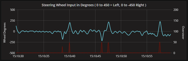
This data is plotted on the Y axis (we're talking graphs now) on the "Steering inputs" panel in Grafana. The oversteer metric can be seen in red and will spike when steering input exceeds 180 degrees in either direction.

Braking too Hard?

Another anomaly I'd like to detect is when maximum brake pressure is applied for too long. Much like the brake pedal in a real car, the brake pedal I'm using has a very progressive feel, a fair amount of force from your foot is required to hit maximum pressure. If you do hit maximum pressure, it shouldn't be for long as you will most likely lock the wheels and skid off the race track, very embarrassing indeed.

The first thing to do is to create a table that will store the last time maximum brake pressure was applied. This table is based on the brake_inputs stream and filters where the value = 100

CREATE TABLE max_brake_power_time \
WITH (kafka_topic = 'max_brake_power_time') AS \
SELECT  axis, \
        MAX(timestamp) as last_max_brake_ts \
FROM    brake_inputs \
WHERE 	value = 100 \
GROUP by axis;

A query of this table displays a new row each time maximum brake pressure is hit.

ksql> SELECT axis, last_max_brake_ts FROM max_brake_power_time;
 Y | 1508769263100
 Y | 1508769267881
 Y | 1508769271568

Something worth mentioning is that if I hold my foot on the brake pedal at the maximum pressure for any period of time, only one event is found in the stream. This is because the device only streams data when the state of an axis changes. If I keep my foot still, no new events will appear in the stream. I'll deal with this in a minute.

Next we'll create a new stream based on the brake_inputs stream and join it to our max_brake_power_time table.

CREATE STREAM brake_inputs_with_max_brake_power_time \
WITH ( kafka_topic = 'brake_inputs_with_max_brake_power_time') AS \
SELECT  bi.value, \
        bi.timestamp, \
        mb.last_max_brake_ts, \
        bi.timestamp - mb.last_max_brake_ts AS time_since_max_brake_released \
FROM    brake_inputs bi LEFT JOIN max_brake_power_time mb ON bi.axis = mb.axis;

For each row in this stream we now have access to all columns in the brake_inputs stream plus a timestamp telling us when max brake power was last reached. With this data we create a new derived column bi.timestamp - mb.last_max_brake_ts AS time_since_max_brake_released which gives a running calculation of the difference between the current record timestamp and the last time maximum brake pressure was applied

For example, when we query the stream we can see that maximum pressure was applied at timestamp 1508772739115 with a value of 100.0. It's the row immediately after this row that we're are interested in 99.90234225 | 1508772740803 | 1508772739115 | 1688.

Again, I've manually added column headings to make it easier to read.

ksql> SELECT value, timestamp, last_max_brake_ts, time_since_max_brake_released FROM brake_inputs_with_max_brake_power_time;

BRAKE VALUE | TIMESTAMP     | LAST MAX BRAKE TIME | TIME SINCE MAX BRAKE RELEASED
98.53513389 | 1508772739100 | 1508772733146       | 5954
98.82810711 | 1508772739100 | 1508772733146       | 5954
99.02342259 | 1508772739115 | 1508772733146       | 5969
99.51171129 | 1508772739115 | 1508772733146       | 5969
99.70702677 | 1508772739115 | 1508772733146       | 5969
100.0       | 1508772739115 | 1508772733146       | 5969
99.90234225 | 1508772740803 | 1508772739115       | 1688
99.51171129 | 1508772740818 | 1508772739115       | 1703
99.12108033 | 1508772740818 | 1508772739115       | 1703
97.65621423 | 1508772740818 | 1508772739115       | 1703
96.58197909 | 1508772740818 | 1508772739115       | 1703
95.41008621 | 1508772740818 | 1508772739115       | 1703
94.43350881 | 1508772740818 | 1508772739115       | 1703
93.65224689 | 1508772740818 | 1508772739115       | 1703
93.35927367 | 1508772740818 | 1508772739115       | 1703
92.87098496 | 1508772740834 | 1508772739115       | 1719
92.38269626 | 1508772740834 | 1508772739115       | 1719
91.11314564 | 1508772740834 | 1508772739115       | 1719
90.62485694 | 1508772740834 | 1508772739115       | 1719
90.42954146 | 1508772740834 | 1508772739115       | 1719
89.35530632 | 1508772740834 | 1508772739115       | 1719
87.89044022 | 1508772740834 | 1508772739115       | 1719
87.40215152 | 1508772740850 | 1508772739115       | 1735
86.52323186 | 1508772740850 | 1508772739115       | 1735

Remember, that while an axis is held at the same value, 100.0 in this case, no more events will appear in the stream until the value changes again. This is why we are interested in the row preceding the maximum value, this row is telling us how long the value of 100.0 was applied for. In this case the time it was held for was 1688 milliseconds. Notice that on subsequent rows the value increases, but we are not interested in those rows. In order to isolate what we want, we need another table. This new table takes our previously created stream, brake_inputs_with_max_brake_power_time and groups it by the last_max_brake_ts column. For each grouping we then get the MIN(time_since_max_brake_released).

CREATE TABLE hard_braking WITH ( kafka_topic = 'hard_braking') AS \
SELECT  last_max_brake_ts, \
        MIN(time_since_max_brake_released) AS time_spent_at_max_brake_ms \
FROM    brake_inputs_with_max_brake_power_time \  
GROUP BY last_max_brake_ts;

When we query this table, while stepping hard on the brake pedal for a few seconds at a time, we get the information we want. We can see the timestamp for when maximum brake pressure reached and for how long it was sustained.

ksql> SELECT last_max_brake_ts, time_spent_at_max_brake_ms FROM hard_braking;
1508775178693 | 1360
1508775178693 | 1360
1508775183334 | 1000
1508775183334 | 1000
1508775187709 | 422
1508775187709 | 422
1508775187709 | 422
1508775187709 | 422
1508775187709 | 422
1508775187709 | 422
1508775187709 | 422
1508775191256 | 1344
1508775191256 | 1344
1508775191256 | 1344
1508775195850 | 1687
1508775195850 | 1687
1508775195850 | 1687
1508775200662 | 1922
1508775200662 | 1922
1508775200662 | 1922
1508775200662 | 1922

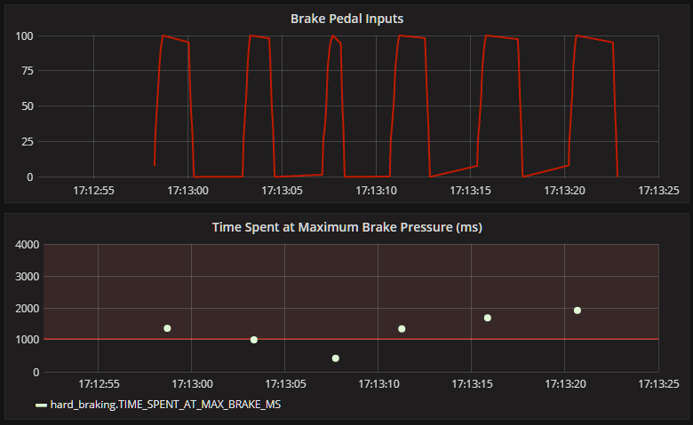
Here's what the above data looks like when visualised in Grafana. The bottom graph is showing when maximum brake pressure was hit and on for how long it was sustained. I've set a threshold against the graph of 1 second so any extreme braking is clearly identifiable - if you're that hard on the brakes for that long, you're probably going to end up in the scenery.

The Tale of 2 Laps

After putting it all together, it's time to take to the track and see how it looks. This video shows 2 complete laps onboard with the Caterham Seven 620R around Brands Hatch in the UK. The first lap is a relatively smooth one and the second is quite ragged. Notice that the first lap ( lap 68 ) is quicker overall than the second ( lap 69 ). On lap 69, I start to drive more aggressively and oversteer spikes start to appear in the steering input graph. Lap 69 also has significantly more events overall than lap 68 as a result my more exuberant ( slower ) driving style. You'll also notice that maximum brake pressure is reached a couple of times on each lap, but for no longer than the threshold of 1 second on each occurrence.

Summary

KSQL is awesome! Although it's only a developer preview at this point, it's impressive what you can get done with it. As it evolves over time and mirrors more of the functionality of the underlying Streams API it will become even more powerful, lowering the barrier to entry for real-time stream processing further and further. Take a look at the road map to see what may be coming next.

Oh, and I recently discovered on the #KSQL community Slack group, that you can execute KSQL in Embedded Mode right inside your Java code, allowing you to mix the native Streams API with KSQL - very nice indeed !