Democratize Data Science with Oracle Analytics Cloud - Data Analysis and Machine Learning

Welcome back! In my previous Post, I described how the democratization of Data Science is a hot topic in the analytical industry. We then explored how Oracle Analytics Cloud can act as an enabler for the transformation from Business Analyst to Data Scientist and covered the first steps in a Data Science project: problem definition, data connection & cleaning. In today's post, we'll cover the second part of the path: from the data transformation and enrichment, the analysis, the machine learning model training and evaluation. Let's Start!
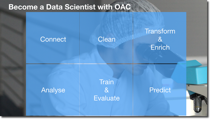
Step #3: Transform & Enrich
In the previous post, we understood how to clean data in order to handle wrong values, outliers, perform aggregation, feature scaling and divide our dataset between train and test. Cleaning the data, however, is only the first step in data processing, and should be followed by what in Data Science is called Feature Engineering.
Feature Engineering is a fancy name to call what in ETL terms we always called data transformation, we take a set of columns in input and we apply transformation rules to create new columns. The aim of Feature Engineering is to create good predictors for the following machine learning model. Feature Engineering is a bit of black art and to achieve excellent results requires a deep understanding of the ML Model we intend to use. However, most of the basic transformations are actually driven by domain knowledge: we should create new columns that we think will improve the problem explanation. Let's see some examples:
- If we're planning to predict the Taxi Fare in New York between any two given points and we have source and destination, a good predictor for the fare probably would be the Euclidean distance between the two.
- If we have Day/Month/Year on separate columns, we may want to condense the information in a unique column containing the Date
- In case our dataset contains location names (Cities, Regions, Countries) we may want to geo-tag those properly with ZIP codes or ISO Codes.
- If we have personal information like Credit Cards details or Person Name, we may want to decide to obfuscate or extract features like the person's sex from the name (on this topic please check the blog post about GDPR and ML from Brendan Tierney).
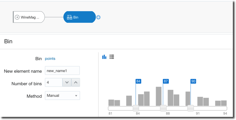
- If we have continuous values like the person's age, do we think there is much difference between a 35, 36 or 37 year-old person? If not we should think about binning them in the same category.
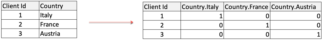
- Most Machine Learning Models can't cope with categorical data, thus we need to transform them to numbers (aka encoding). The standard process, when no ordering exists between the labels, is to create a new column for each value and mark the rows with
1/0accordingly.
Oracle Analytics Cloud again covers all the above cases with two tools: Euclidean distance, generic data transformation like data condensation and binning are standard steps of the Dataflow component. We only need to set the correct parameters or write simple SQL-like statements. Moreover, for binning, there are options to do it manually as well as automatically providing equal-width and equal-height bins therefore taking out the manual labour and related BIAS.
On the other side the geo-tagging, data obfuscation, automatic feature extraction (like person's sex based on name) is something that with most of the other tools needs to be resolved by hand, with complex SQL statements or dedicated Machine Learning efforts.
OAC again does a great job during the Data Preparation Recommendation step: after defining a data source, OAC will scan column names and values in order to find interesting features and propose some recommendations like geo-tagging, obfuscation, data splitting (e.g. Full Name split into First and Last Name) etc.
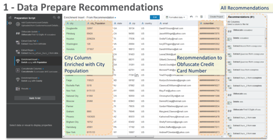
The accepted recommendations will be added to a Data Preparation Script that can be automatically applied when updating our dataset.
Step #4: Data Analysis
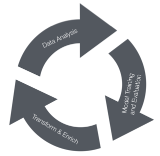
Data Analysis is declared as Step #4 however since the Data Transformation and Enrichment phase we started a circular flow in order to optimize our predictive model output.
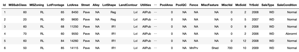
The analysis is a crucial step for any Data Science project; in R or Python one of the first steps is to check dataset head() that will show a first overview of the data like the below
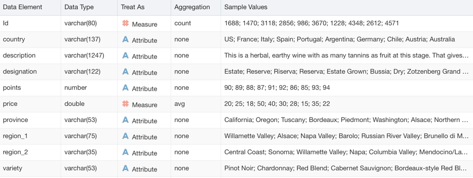
OAC does a similar job with the Metadata Overview where we can see for each column the name, type and sample values as well as the Attribute/Metric definition and associated aggregation than we can then change later on.
Analysing Data is always a complex task and is where the expert eye of a data scientist makes the difference. OAC, however, can help with the excellent Explain feature. As described in the previous post, by right clicking on any column in the dataset and selecting Explain, OAC will start calculating statistics and metrics related to the column and display the findings in graphs that we can incorporate in the Data Visualization project.
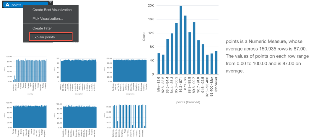
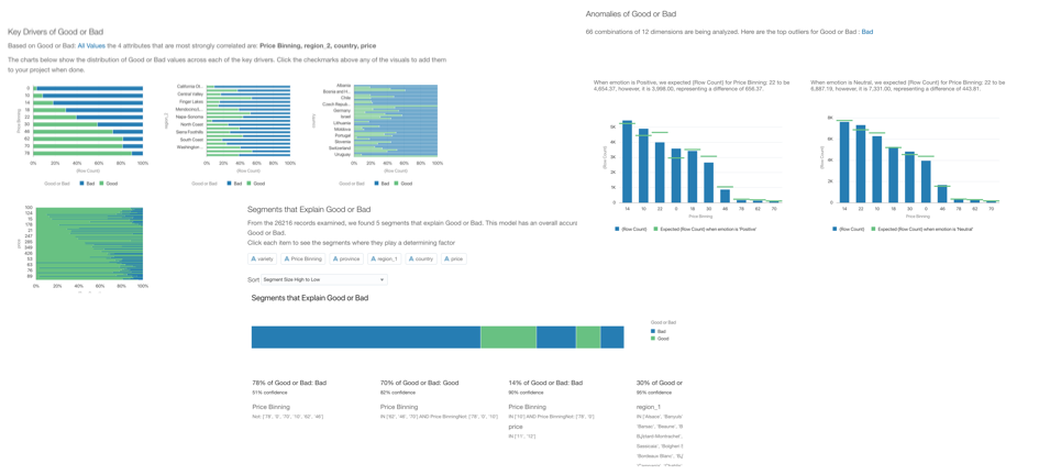
Even more, there are additional tabs in the Explain window that provide Key Drivers, Segments and Anomalies.
- Key Drivers provides the statistically significant drivers for the column we are examining.
- Segments shows hidden groups in the dataset that can predict outcomes in the column
- Anomalies does an outlier detection, showing which are corner cases in our dataset
Some Data Science projects could already end here. If the objective was to find insights, anomalies or particular segments in our dataset, Explain already provides that information in a clear and reusable format. We can add the necessary visualization to a Project and create a story with the Narrate option.
If on the other side, our scope is to build a predictive model, then it's time to tackle the next phase: Model Training & Evaluation.
Step #5: Train & Evaluate
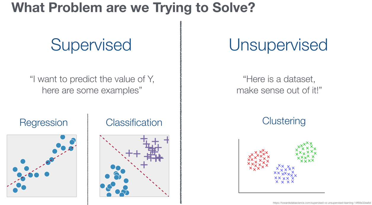
Exciting: now it's time to tackle Machine Learning! The first thing to do is to understand what type of problem we are trying to solve. OAC allows us to solve problems in the following categories:
- Supervised when we have a history of the problem's solution and we want to predict future outcomes, we can then identify two subcategories
- Regression when we are trying to predict a continuous numerical value
- Classification when we are trying to assign every sample to a category out of two or more
- Unsupervised when we don't have a history of the solution, but we ask the ML tool to help us understanding the dataset.
- Clustering when we try to label our dataset in categories based on similarity.
OAC provides two different ways to apply Machine Learning on a dataset: On the Fly or via DataFlows. The On the Fly method is provided directly in the data visualization: when we create any chart, OAC provides the option to add Clusters, Outliers, Trend and Forecast Lines.
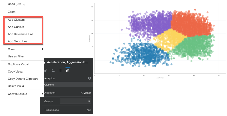
When adding one of the Analytics, we have some control over the behaviour of the predictive model. For the clustering image above we can decide which algorithm to implement (between K-means and Hierarchical Clustering), the number of clusters and the trellis scope in case we visualize multiple scatterplots, one for each value of a dimension.
Applying Machine Learning models on the fly is very useful and could provide some great insights, however, it suffers from a limitation: the columns analysed by the model are only the ones included in the visualization, we have no control over other columns we may want to add to the model to increase predictions accuracy.
If we want to have granular control over columns, algorithm and parameters to use, OAC provides the Train Model step in the DataFlow component.

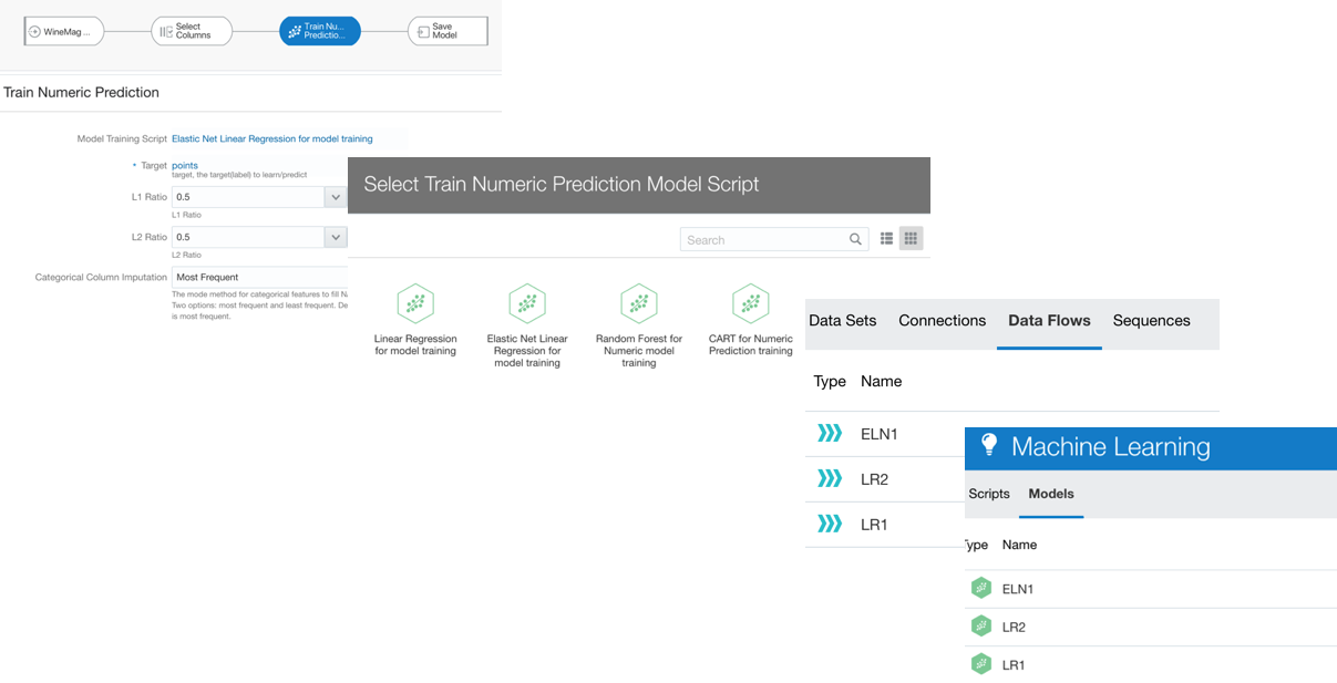
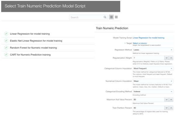
As described above OAC provides the option to solve Regression problems via Numeric Prediction, apply Binary or Multi-Classifier for Classification, and Clustering. There is also an option to train Custom Models which can be scripted by a Data Scientist, wrapped in XML tags and included in OAC (more about this topic in a later post).
Once we've selected the class of problem we're aiming to solve, OAC lets us select which Model to train between various prebuilt ones. After selecting the model, we need to identify which is the target column (for Supervised ML classes) and fix the parameters. Note the Train Partition Percent providing an automated way to split the dataset in train/test and Categorical/Numerical Column Imputation to handle the missing values. As part of this process, the encoding for categorical data is executed.
... But which Model should we use? What parameters should we pick? One lesson I got from my knowledge of Machine Learning is that there is no golden model and parameters set to solve all problems. Data Scientist will try to use different models, compare them and tune parameters based on experimentation (aka trial and error).
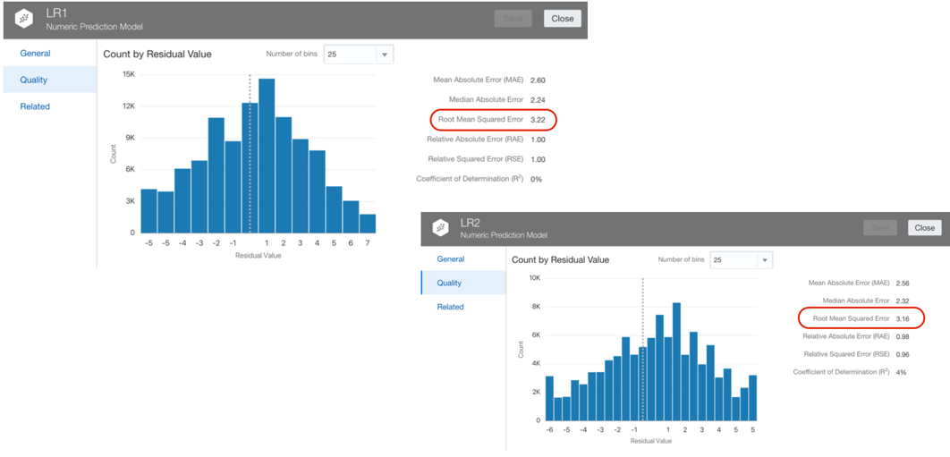
OAC allows us to create an initial Dataflow, select a model, set the parameters then save the Dataflow and model output. Then restart by opening the Dataflow changing the model or the parameters and storing the artefacts with different names to compare them.

After creating one or more Models, it's time to evaluate them, on OAC we can select a Model and Click on Inspect. In the Overview tab, Inspect shows the model description and properties. Far more interesting is the Quality tab which provides a set of Model scoring metrics based on the test dataset created following the Train Partition Percent parameter. In case of a Numeric Prediction problem, the Quality tab will show for each model quality metrics like the Root Mean Squared Error. OAC will provide similar metrics no matter which ML algorithm you're implementing, making the analysis and comparison easy.
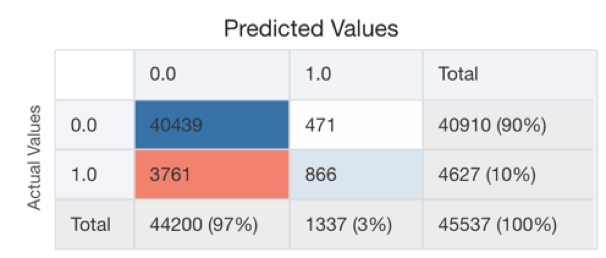
In the case of Classification, the Quality Tab will show the confusion matrix together with some pre-calculated metrics like Precision, Recall etc.
The model selection then becomes an optimization problem for the metric (or set of) we picked during the problem definition (see TEP in the previous post). After trying several models, parameters, features, we'll then choose the model that minimizes the error (or increase the accuracy) of our prediction.
Note: as part of the model training, it's very important to select which columns will be used for the prediction. A blind option is to use all columns but adding irrelevant columns isn't going to provide better results and, for big or wide (huge number of columns) datasets, it becomes computationally very expensive. As written before, the Explain function provides the list of columns that represent statistically significant predictors. The columns listed there should represent the basics of the model training.
Ok, part II done, we saw how to perform Feature Engineering and Model Training and Evaluation, check my next post for the final piece of the Data Science journey: Predictions and final considerations!
Edit: Link to Part III of the series.