Joining Data in OAC

One of the new features in OAC 6.0 was Multi Table Datasets, which provides another way to join tables to create a Data Set.

We can already define joins in the RPD, use joins in OAC’s Data Flows and join Data Sets using blending in DV Projects, so I went on a little quest to compare the pros and cons of each of the methods to see if I can conclude which one works best.

What is a data join?

Data in databases is generally spread across multiple tables and it is difficult to understand what the data means without putting it together. Using data joins we can stitch the data together, making it easier to find relationships and extract the information we need. To join two tables, at least one column in each table must be the same. There are four available types of joins I’ll evaluate:

1.    Inner join - returns records that have matching values in both tables. All the other records are excluded.

2.    Left (outer) join - returns all records from the left table with the matched records from the right table.

3.    Right (outer) join - returns all records from the right table with the matched records from the left table.

4.    Full (outer) join - returns all records when there is a match in either left or right tables.

Each of the three approaches give the developer different ways and places to define the relationship (join) between the tables. Underpinning all of the approaches is SQL. Ultimately, OAC will generate a SQL query that will retrieve data from the database, so to understand joins, let’s start by looking at SQL Joins

SQL Joins

In an SQL query, a JOIN clause is used to execute this function. Here is an example:

SELECT EMP.id, EMP.name, DEPT.stream
FROM EMP
INNER JOIN DEPT ON DEPT.id = EMP.id;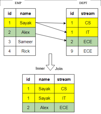  

Now that we understand the basic concepts, let’s look at the options available in OAC.

Option 1: RPD Joins

The RPD is where the BI Server stores its metadata. Defining joins in the RPD is done in the Admin Client Tool and is the most rigorous of the join options. Joins are defined during the development of the RPD and, as such, are subject to the software development lifecycle and are typically thoroughly tested.

End users access the data through Subject Areas, either using classic Answers and Dashboards, or DV. This means the join is automatically applied as fields are selected, giving you more control over your data and, since the RPD is not visible to end-users, avoiding them making any incorrect joins.

The main downside of defining joins in the RPD is that it’s a slower process - if your boss expects you to draw up some analyses by the end of the day, you may not make the deadline using the RPD. It takes time to organise data, make changes, then test and release the RPD.

Join Details

The Admin Client Tool allows you to define logical and physical tables, aggregate table navigation, and physical-to-logical mappings. In the physical layer you define primary and foreign keys using either the properties editor or the Physical Diagram window. Once the columns have been mapped to the logical tables, logical keys and joins need to be defined. Logical keys are generally automatically created when mapping physical key columns. Logical joins do not specify join columns, these are derived from the physical mappings.

You can change the properties of the logical join; in the Business Model Diagram you can set a driving table (which optimises how the BI Server process joins when one table is smaller than the other), the cardinality (which expresses how rows in one table are related to rows in the table to which it is joined), and the type of join.

Driving tables only activate query optimisation within the BI Server when one of the tables is much smaller than the other. When you specify a driving table, the BI Server only uses it if the query plan determines that its use will optimise query processing. In general, driving tables can be used with inner joins, and for outer joins when the driving table is the left table for a left outer join, or the right table for a right outer join. Driving tables are not used for full outer joins.

The Physical Diagram join also gives you an expression editor to manually write SQL for the join you want to perform on desired columns, introducing complexity and flexibility to customise the nature of the join. You can define complex joins, i.e. those over non-foreign key and primary key columns, using the expression editor rather than key column relationships. Complex joins are not as efficient, however, because they don’t use key column relationships.

It’s worth addressing a separate type of table available for creation in the RPD – lookup tables. Lookup tables can be added to reference both physical and logical tables, and there are several use cases for them e.g., pushing currency conversions to separate calculations. The RPD also allows you to define a logical table as being a lookup table in the common use case of making ID to description mappings.

Lookup tables can be sparse and/or dense in nature. A dense lookup tables contains translations in all languages for every record in the base table. A sparse lookup table contains translations for only some records in the base tables. They can be accessed via a logical calculation using DENSE or SPARSE lookup function calls. Lookup tables are handy as they allow you to model the lookup data within the business model; they’re typically used for lookups held in different databases to the main data set.

Multi-database joins allow you to join tables from across different databases. Even though the BI Server can optimise the performance of multi-database joins, these joins are significantly slower than those within a single database.

Option 2: Data Flow Joins

Data Flows provide a way to transform data in DV. The data flow editor gives us a canvas where we can add steps to transform columns, merge, join or filter data, plot forecasts or apply various models on our datasets.

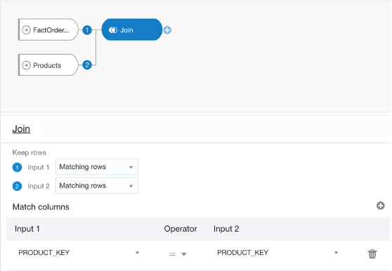
When it comes to joining datasets, you start by adding two or more datasets. If they have one or more matching columns DV automatically detects this and joins them; otherwise, you have to manually add a ‘Join’ step and provided the columns’ data types match, a join is created.

A join in a data flow is only possible between two datasets, so if you wanted to join a third dataset you have to create a join between the output of the first and second tables and the third, and so on. You can give your join a name and description which would help keep track if there are more than two datasets involved. You can then view and edit the join properties via these nodes created against each dataset. DV gives you the standard four types of joins (Fig. 1), but they are worded differently; you can set four possible combinations for each input node by toggling between ‘All rows’ and ‘Matching rows’. That means:

The table above explains which type of join can be achieved by toggling between the two drop-down options for each dataset in a data flow join.

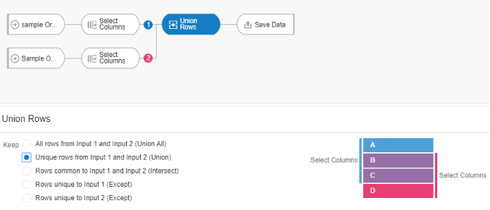
It’s worth mentioning there is also an operator called ‘Union Rows’. You can concatenate two datasets, provided they have the same number of columns with compatible datatypes. There are a number of options to decide how you want to combine the rows of the datasets.

One advantage of data flows is they allow you to materialise the data i.e. save it to disk or a database table. If your join query takes 30 minutes to run, you can schedule it to run overnight and then reports can query the resultant dataset.

However, there are limited options as to the complexity of joins you can create:

1. the absence of an expression editor to define complex joins
2. you cannot join more than two datasets at a time.

You can schedule data flows which would allow you to materialise the data overnight ready for when users want to query the data at the start of the day.

Data Flows can be developed and executed on the fly, unlike the longer development lifecycle of the RPD.

It should be noted that Data Flows cannot be shared. The only way around this is to export the Data Flow and have the other user import and execute it. The other user will need to be able to access the underlying Data Sets.

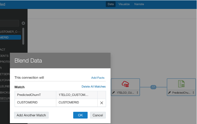
Option 3: Data Blending

Before looking at the new OAC feature, there is a method already present for cross-database joins which is blending data.

Given at least two data sources, for example, a database connection and an excel spreadsheet from your computer, you can create a Project with one dataset and add the other Data Set under the Visualise tab. The system tries to find matches for the data that’s added based on common column names and compatible data types. Upon navigating back to the Data tab, you can also manually blend the datasets by selecting matching columns from each dataset. However, there is no ability to edit any other join properties.

Option 4: Multi Table Datasets

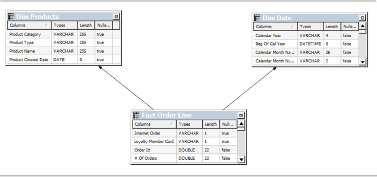
Lastly, let’s look at the newly added feature of OAC 6.0: Multi Table Datasets. Oracle have now made it possible to join several tables to create a new Data Set in DV.

Historically you could create Data Sets from a database connection or upload files from your computer. You can now create a new Data Set and add multiple tables from the same database connection. Oracle has published a list of compatible data sources.

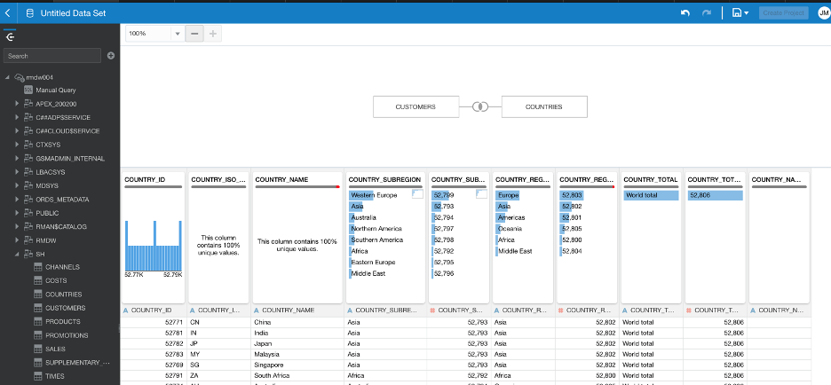
Once you add your tables DV will automatically populate joins, if possible, on common column names and compatible data types.

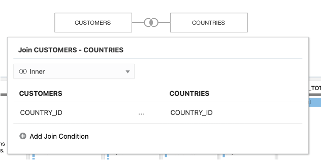
The process works similarly to how joins are defined in Data Flows; a pop-up window displays editable properties of the join with the same complexity - the options to change type, columns to match, the operator type relating them, and add join conditions.

The data preview refreshes upon changes made in the joins, making it easy to see the impact of joins as they are made.

Unlike in the RPD, you do not have to create aliases of tables in order to use them for multiple purposes; you can directly import tables from a database connection, create joins and save this Multi Table Dataset separately to then use it further in a project, for example. So, the original tables you imported will retain their original properties.

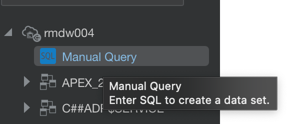
If you need to write complex queries you can use the Manual SQL Query editor to create a Data Set, but you can only use the ‘JOIN’ clause.

So, what’s the verdict?

Well, after experimenting with each type of joining method and talking to colleagues with experience, the verdict is: it depends on the use case.

There really is no right or wrong method of joining datasets and each approach has its pros and cons, but I think what matters is evaluating which one would be more advantageous for the particular use case at hand.

Using the RPD is a safer and more robust option, you have control over the data from start to end, so you can reduce the chance of incorrect joins. However, it is considerably slower and make not be feasible if users demand quick results. In this case, using one of the options in DV may seem more beneficial.

You could either use Data Flows, either scheduled or run manually, or Multi Table Datasets. Both approaches have less scope for making complex joins than the RPD. You can only join two Data Sets at a time in the traditional data flow, and you need a workaround in DV to join data across database connections and computer-uploaded files; so if time and efficiency is of essence, these can be a disadvantage.

I would say it’s about striking a balance between turnaround time and quality - of course both good data analysis in good time is desirable, but when it comes to joining datasets in these platforms it will be worth evaluating how the use case will benefit from either end of the spectrum.

Find out more about joining data in OAC - contact the Rittman Mead team.