Giving OAC Semantic Modeler a Try

Kids just love it when old folk go on about good old days. The particular good old days I have in mind is when Oracle CRM On Demand was released. Competition in the Cloud CRM space was tough but the Oracle product had one trick up its sleeve: its data analytics capability that set it apart from the competition. It was almost scary how well CRM worked in the cloud, and Cloud BI surely was just round the corner. A few years later (time seems to pass quicker as you get older), Oracle Analytics Cloud (OAC) gets released and we can safely say that Cloud BI works. The Semantic Modeler that has been made available for evaluation on May 2022 as part of OAC, is a big step towards Cloud BI not just working but working well.

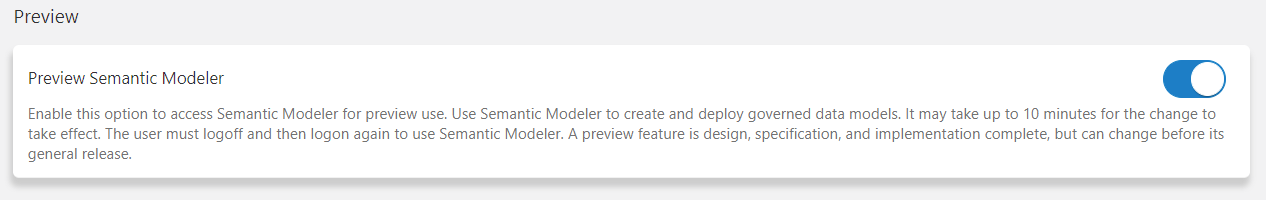
At the time of this writing, Semantic Modeler is available for evaluation only, hence needs to be enabled from the Navigator menu > Console > System Settings > Preview Semantic Modeler.

Once enabled, we are ready to try it out, to see how it compares to the old ways.

From the Create menu we select Semantic Model and choose to start with an empty Model.

Let us call our Model 'HelloSemanticModel'. Once it is created, its high-level building blocks are available as icons just under the Model name:

1. Connections,
2. Physical Layer,
3. Logical Layer,
4. Presentation Layer,
5. Variables,
6. Invalid Files.

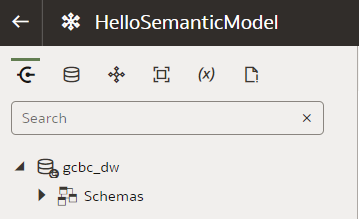
The names of items 2., 3. and 4. look familiar - indeed they are borrowed from the three Layers of the OBIEE's RPD.

Semantic Model's Physical Layer

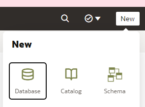
Here we manage Databases that consist of Physical Schemas, Tables, Table Aliases and Joins between them - much like in the RPD's Physical Layer. Let us create a new Database - from the New menu we select Database.

Interestingly, the Physical Layer is not where physical database connections are defined - they are defined outside the Semantic Model. But Connections are visible in the Semantic Modeler's Connections view - this is where we select a FACT table and drag and drop it into our newly created Database's Tables view. Helpfully, it offers to import the DIMs that are joined to it in the physical database and even creates joins.

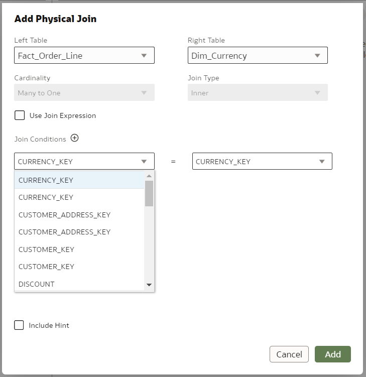
However, the joins created are of little use to us - our FACT_ORDER_LINE fact joins to the DIM_ADDRESS dimension in 3 ways: as Customer, Outlet and Staff Address. Just like in the RPD, we fix that by using Table Aliases.

After creating Aliases for all Physical Tables, I was about to create Joins between them and then I saw this:

Columns in all my Physical Tables had been duplicated. Why? Because most of my Aliases were named the same as their base Physical Tables, the only difference being UPPER_CASE replaced with Camel_Case. It turns out, Semantic Modeler's name uniqueness checker is case sensitive whereas further down the line the case is ignored. The best way I found to fix this was to scrap and re-create the Semantic Model, while reminding myself this is just a preview.

After re-creating the Model and using proper naming for Aliases, the issue was fixed.

Before moving on to the next Layer, let us have a look at the Connection Pool tab. Instead of defining a connection from start to finish like in the RPD, here you select it from a drop-down and provide a bit of additional info like Timeout and DB Writeback.

Semantic Model's Logical Layer

Semantic Model's Logical Layer does the same job as the RPD's BMM Layer. Here, as expected, we turn Physical Database Tables into Facts and Dimensions and define Logical Joins between them. Lookup Tables don't get to hang out with the cool guys - they are separated from Facts and Dimensions in a different tab.

Do you notice something missing? That's right - no dimension hierarchies! That is because they are now part of the Dimension tables, which makes sense.

First we import the Fact table. Then the Dimensions. Helpfully, the dimensions that the Fact table can physically be joined with, are already pre-selected.

After importing the Dimensions, we want to define their Hierarchies.  To do that, we have to right-click on each and choose Edit from the menu.

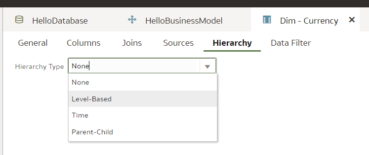
Then we go straight to the Hierarchy tab and define a Dimensional Hierarchy in a manner very similar to RPD.

Grand total:

Detail:

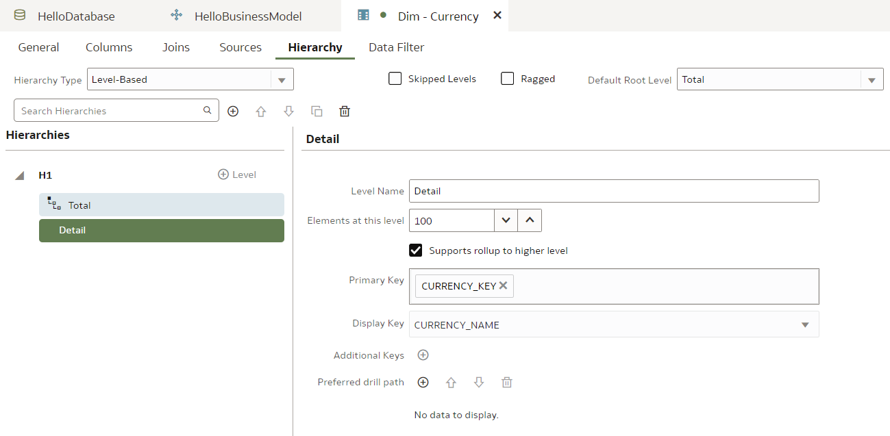
It looks very similar to RPD so we feel right at home here. (To build an entire Model in a single blog post, we rush forward without exploring the detail.)

Now that dimensional hierarchies are defined, we want to set dimensional levels for our Fact Source. We right-click our Fact table and choose Edit from menu.

We scroll down the Sources tab and, unsurprisingly, we find Data Granularity section. Setting dimensional levels here is nicer than in the RPD's Admin Tool - kids have it so easy these days!

Before we move on to the next Layer, let us have a look at Attribute expressions. We create a Full Name attribute for the Dim - Customers dimension as a concatenation of First and Last Names.

Notice the Aggregation Rule option here, relevant for facts.

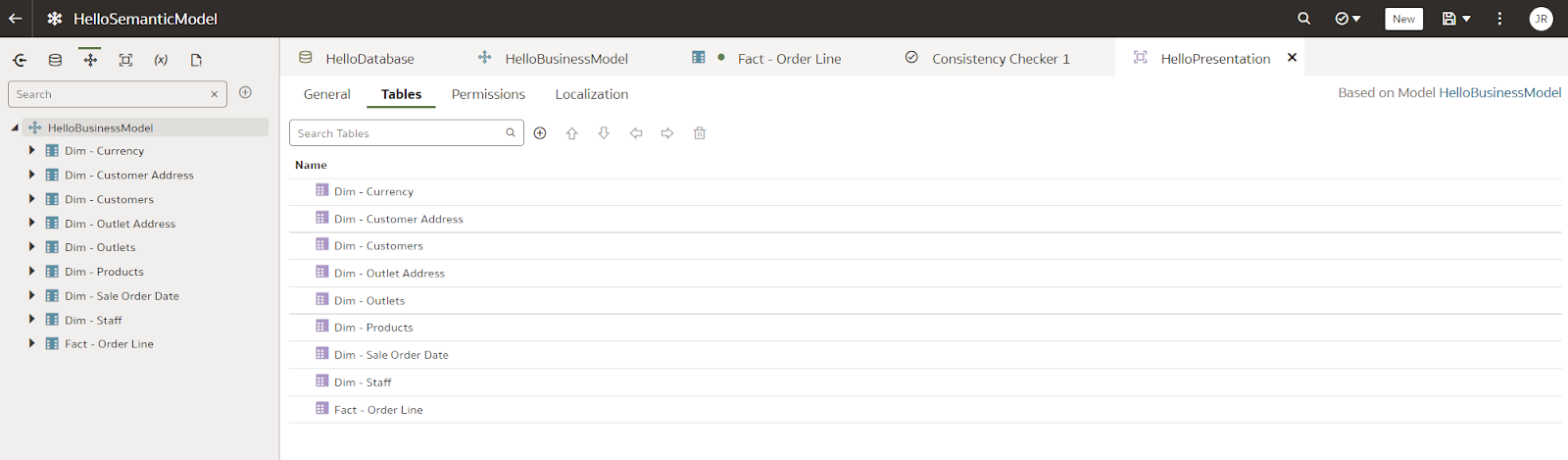
Semantic Model's Presentation Layer

Not much going on here - we create a Subject Area...

... and add tables to it.

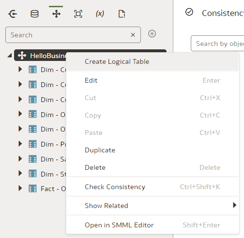
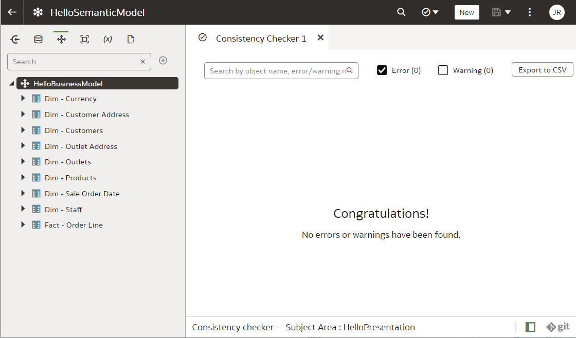
All done!  Well, almost. Just like in the Admin Tool, we want to check consistency.

Is Cloud BI the Future?

It has been a long wait but now it looks like it! Whilst not perfectly stable and production-ready, using the Semantic Modeler is a good experience. In this blog post we went through the creation of a very simple dimensional model. I did not mention the very promising lineage visualisation capability that the Semantic Modeler now offers, the new and much nicer SMML language instead of the old UDML language of the OBIEE's RPD, Git support. But those are so exciting they deserve their own blog posts. The future looks bright for Cloud BI. Back in the day when we worked with Siebel Analytics, we could only dream of...