Breaking the Assumptions of Linear Regression
Linear Regression must be handled with caution as it works on five core assumptions which, if broken, result in a model that is at best sub-optimal and at worst deceptive.

Introduction
The Linear Model is the most commonly-used tool in machine learning, and for a good reason: it remains a powerful tool for producing interpretable predictions, it requires less data pre-processing than many other models and it is robust against overfitting. Advantages aside, Linear Regression must be handled with caution as it works on five core assumptions which, if broken, result in a model that is at best sub-optimal and at worst deceptive. It's tempting to save time by not bothering to check these assumptions, but ultimately it is better to be in the habit of checking these assumptions whenever a Linear Model is employed, and once you get into the habit of running these checks you'll find that they don't take so long after all.
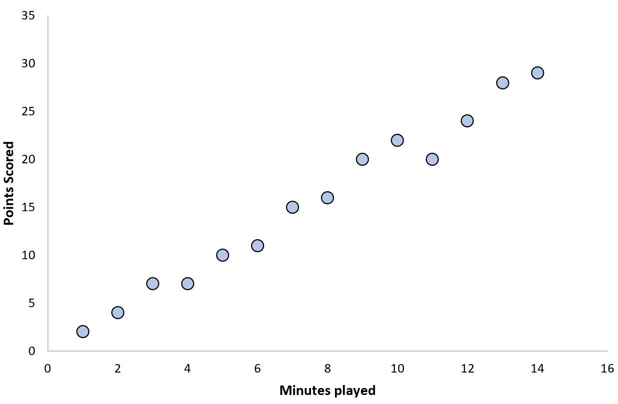
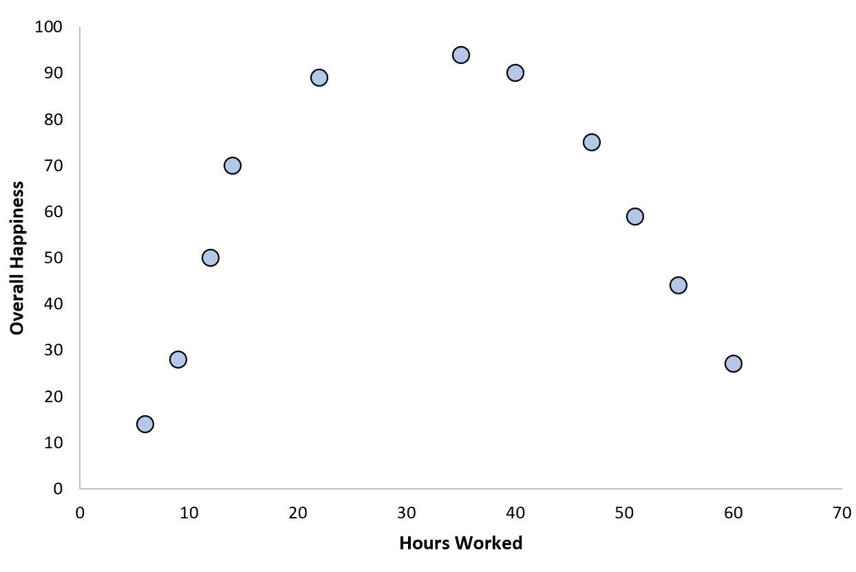
Assumption 1: Linearity
This one is fairly straightforward: Linear Regression assumes a Linear Relationship. The way to test a linear relationship is to create a scatterplot of your variables and check whether the relationship looks linear (i.e. a straight line). If the regression line is curved or if there is no clear line then there is likely no linear relationship. This assumption can also be violated by outliers, so checking for these is important.
How to deal with nonlinearity
Using a non-linear model may work better for this kind of data.
If it's broken...
Of all the five assumptions, this may be the absolute worst one to break. When you break this assumption it is rare for it not to cause serious errors in the insights drawn from the data.
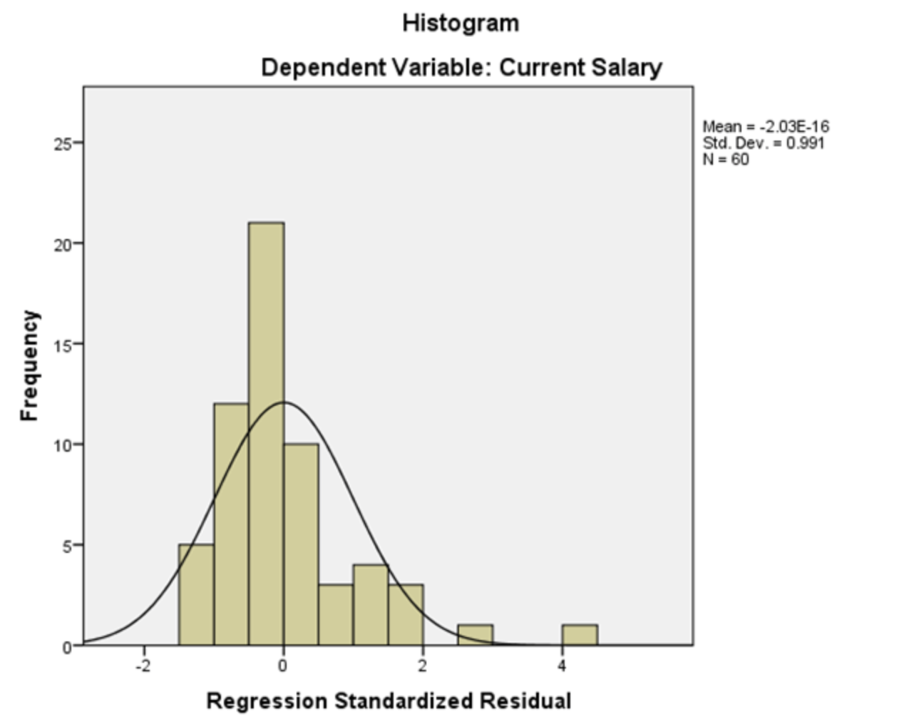
Assumption 2: Normality
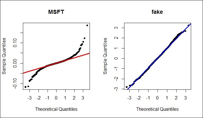
This assumption is that The errors (residuals) of your model should follow a normal distribution (this does not mean that the independent variables must follow a normal distribution; only that the errors need to). This assumption is harder to grasp intuitively. One way to think about this assumption is that we should expect smaller errors to be reasonably more common than big errors- but not overwhelmingly more common, and we should also expect that big errors are equally likely in either direction, via both overestimating and underestimating the true value. Thankfully this assumption is relatively easy to check: plot the model residuals on a histogram and check if the plot looks like a normal bell curve. If you're not sure, make a Q-Q plot.
How to deal with abnormality
A log or a square-root transformation of the data often fixes this issue.
If it's broken...
Violating the assumption of normality is not that bad compared to some of the other assumptions. The risk here is that your confidence intervals may be misleading, either by being too large or too small. This is undesirable, but it is less likely to cause a catastrophe than violating the assumption of linearity.
Assumption 3: No Multicollinearity
Multicollinearity is simple to explain: it is when the Independent Variables (or Features, if you're from a Computer Science background) are too highly-correlated with one another. Multicollinearity is a problem because it reduces the apparent strength of significant variables.
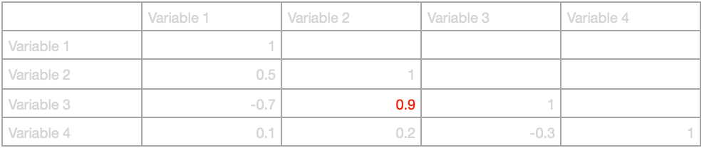
There are several ways to check for multicollinearity, but I find that the simplest method is to use a correlation matrix. Creating a correlation matrix for all of the independent variables will highlight any that are highly-correlated with one another. Typically a correlation of 0.9 or higher is taken as the threshold for multicollinearity, though sometimes 0.8 is used.
How to deal with multicollinearity
The simplest way to deal with multicollinearity is to delete one of the highly-correlated variables. This had the advantage of keeping the rest of the input variables as whatever they originally were, which may help with interpretability.
Another option could be to run a Principal Component Analysis and turn the two highly-correlated variables into a single variable. This has the disadvantage of requiring careful labelling and interpretation of this new variable, potentially leading to incorrect conclusions when interpreting the model's coefficients.
If it's broken...
Multicollinearity is more of a problem for inference than prediction, because the final prediction is still going to be the same even with multicollinearity in the independent variables, but the relative contributions of each variable will be misleading for the purpose of inferring their relative impacts.
Assumption 4: Independence of Errors
This is the hardest assumption to get an intuitive understanding for. This assumption says that The errors for one variable should not correlate with the errors for another. This assumption is one of the trickiest to test for and its violation can mean several different possible things. Non-independent errors tend to be a bigger problem when considering time-series data, though they can also occur in other kinds of data.
How to deal with non-independence of errors
If you are using time series data, you can check for independence of errors with a Durbin-Watson test. Otherwise, you can check by plotting the errors against one another. If there appears to be a correlation, you likely do not have independence of errors. The fix taken will depend on the result of the test and some trial-and-error. For instance, if you are using a time-series model then you may not have accounted for seasonal variation. An intuitive way to think about independence of errors is that if you find that errors can predict other errors then you should be using that information to reduce the errors; if you know that overestimating a variable today means you're likely to overestimate tomorrow, then you should be accounting for that.
If it's broken...
It is fairly serious when independence of errors is violated. Confidence intervals and significance tests rely on this assumption, so identifying independent variables that impact the dependent variable with statistical significance may be misidentified.
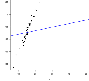
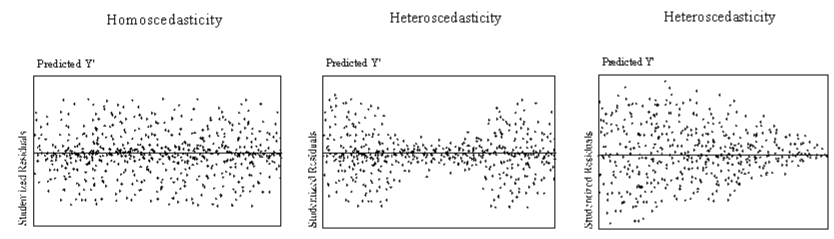
Assumption 5: Homoscedasticity
Homoscedasticity is the assumption that errors do not vary as the dependent variable gets larger or smaller.
How to deal with heteroscedasticity
You can check for heteroscedasticity by plotting the errors against the dependent variable, as pictured above. If you have heteroscedasticity that appears to be linear (such as the plot on the right above), a log transformation may fix it. If you have latent seasonality that hasn't been accounted for, adding a dummy variable for season may fix the heteroscedasticity.
If it's broken...
Heteroscedasticity can cause your model to incorrectly count an independent variable as significant when it is not, or vice versa (though the former is more common). Heteroscedasticity does not introduce bias per se, it just reduces the precision of your estimates.
Conclusion
The linear model is a simple, flexible and powerful tool that will never go out of style, but there have to be drawbacks- otherwise we would not have invented other kinds of models. One of the most overlooked drawbacks of the linear model is its fragility. Other kinds of models will often fail in obvious ways, but a linear model is dangerous because it can easily fail silently.