Retrieval Augmented Generation - A Primer

Retrieval augmented generation, or RAG, is rapidly gaining traction as the next disruptive evolution for generative AI models. Promising a reduction in the hallucinations sometimes experienced by large language models such as GPT-4, greater accuracy of responses, access to up-to-date information, and the capability to use private or proprietary data without exposing those same data to actors outside of one’s organisation, RAG models represent a major increase in capability for over purely generative, pre-trained models such as GPT and LLaMa. With these potential benefits in mind, and with major industry players like Oracle and MongoDB bringing their own RAG-enabled solutions to market, now is a great time to get a top-level understanding of what RAG actually is. In this post, we’re going to walk you through the basics of RAG and the vector database principles that underpin it, covering why it’s useful, how it works, and what limitations it may experience.
Pure Generative Versus RAG
Drawbacks of Current Generative Models
Existing generative AI models such as GPT-4 and LLaMa have captured a lot of interest, both publicly and within the AI community, for their ability to ingest vast quantities of data, learn the syntactic rules of communication, and then capably interpret input queries to return a semantically or stylistically accurate output. While powerful for summarising large corpuses of data in a few paragraphs, or finding a specific piece of information within a sea of data, these models soon hit a few problems on close inspection.
Principal among these problems is the tendency for ‘hallucinations’, when the pre-trained model doesn’t know the answer to an input query and, instead of responding that it doesn’t know, fabricates a convincing-sounding but inaccurate answer. It is primarily this behaviour that led to swift action from Stack Overflow to ban AI-generated answers to user questions, with similar moves from other institutions regarding the usage and trust of Chat-GPT for commercial or official purposes.
Secondly, a pre-trained model only knows about the data on which it was trained. In other words, it rapidly becomes stale when trying to train it to understand current events. The freely available instance of Chat-GPT, for example, uses GPT-3.5, trained on data up to January 2022, and therefore it is unable to answer queries about any events beyond that date. This is obviously problematic when seeking answers about fields which are in ongoing development or see fast-moving change, such as AI, features of programming languages and libraries, legislation and so on. While models can be re-trained, the time taken and compute power required to do this make it prohibitive to perform frequently, and it is only ever a temporary fix.
Finally, pre-trained models do not have access to your organisation's private or proprietary data. This is obviously a good thing for the most part; no one's private information should be publicly exposed via a generative AI model. However, this does mean that the power of a generative model cannot be utilised on private or commercially sensitive information, or that a locked-down instance of the model must be trained on those data, at the cost of time, compute power, and maintenance.
We can really summarise these problems as the issue of hallucinations and two major causes thereof, which combine to become a major limitation of purely generative models. It is in addressing this limitation that RAG demonstrates its value.
Retrieval Augmentation
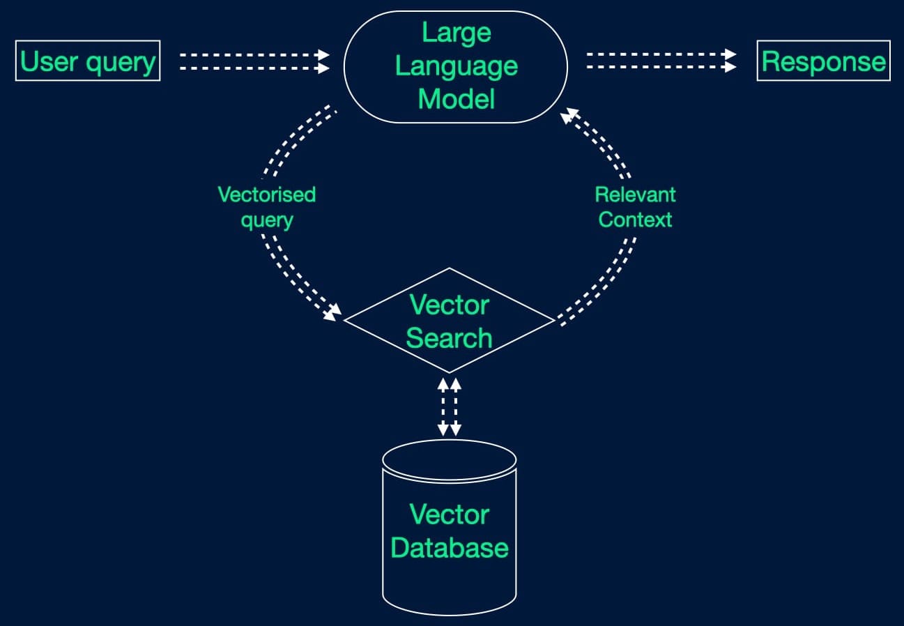
In an impressive feat of appropriate nomenclature, retrieval augmented generation models make use of an information retrieval architecture to augment the generation process. In simple terms, it’s a generative model which uses a search engine, pointed towards a vector database of known-good data, to provide the information and context to answer the query being posed, rather than relying on the information on which it was trained. The consequences of this simple addition are far reaching; by backing the generative model using an arbitrary and private database of information, we can leverage the semantic understanding given by a large language model (LLM) to both interpret the query and construct an answer, while ensuring that we always have the required information available in a non-stale, non-public repository.
The basic process is as follows:
- The user inputs their prompt to the model
- The LLM interprets the query (embedding)
- The retrieval architecture searches the database and returns the relevant information (vector search)
- The LLM uses that information to generate an answer
In principle, RAG is similar to fine-tuning a LLM, but much more powerful. As a reminder, fine-tuning is the insertion of context into the prompts or queries passed to a model; in this way, we’re notionally retraining or providing additional training on top of the base model to include more topics or more private or sensitive data, but this is limited to how much information we can squeeze into the prompt and will be sensitive to the exact wording used. RAG, on the other hand, includes context from your database at the time of inference, and by constructing the prompt well we can even specify that only the context in the database should be used to generate an answer.
So how does this address the hallucination, and causes thereof, that we observed with purely generative models?
With RAG, we can ensure that sensitive and up-to-date information is always available to our model by simply inserting new data into our vector database. We can then tell the model via our input prompt to use only the information in the database to answer our query, with a strict requirement to say ‘I don’t know' if the answer is not explicitly included within that context. This mitigates against hallucinations and allows our model to access new data without costly retraining and without the actual model learning that information. Private data are thereby not made publicly visible via the model, and we improve security and compartmentalisation between users; a user’s credentials and the database management system control which data are visible and queryable by the user, and the model generates a response based on what they are permitted to access.
RAG Pre-processing and Architecture
RAG clearly has a lot to offer as an evolution of generative AI, but doing so requires a few extra pieces of pre-processing and architecture to support the vector database and the data held within. Let’s take a look at what they are and how they work.
Data Chunking
Constructing a vector database for RAG starts, as many things do, with a large volume of unstructured data. This may be a corpus of very many documents, a library of millions of pictures, thousands of hours of video or something else entirely depending on the application. Without loss of generality, we’ll focus on the textual data case, but the principles apply equally to other forms of unstructured data.
A strategy is needed for storing our huge volume of raw data in a way which allows it to be searched for pieces of relevant information, and that strategy is called chunking. In very literal terms, the data are divided up into chunks prior to storage, so that each one can be inspected for relevance to the input query during a search. It is best practice to include some overlap in these chunks, to avoid information being split between chunk boundaries and thereby lost during the chunking process.
The size and format of these chunks can be very different from application to application, and it’s always a balancing act of having small enough chunks that they can be quickly compared to one another, versus large enough chunks that each one contains meaningful information. It’s also important to consider the total number of chunks; create too many, and execution of the model will slow down due to the number of comparisons required when performing a search.
For structured text formats like HTML and JSON, we may be able to take advantage of the inherent formatting hints in the document and chunk on paragraph or heading tags. Longer form prose may simply take a sentence or number of sentences per chunk, and small documents may be a chunk in and of themselves. Optimising the chunk size for the application and platform in question is an important step to achieve the required accuracy and speed.
Vector Embedding
To be able to provide answers in a useful timeframe, RAG must solve the problem of how to rapidly search a database of information on which it was not trained, and return relevant pieces of information from which to construct an answer. Searches of this kind on any kind of unstructured data are non-trivial, so we first must first map those unstructured data to structured numerical vector, in a process known as vector embedding.
Vector embedding represents an arbitrary piece of unstructured data as an n-dimensional array of floats. These numbers may not be inherently meaningful or interpretable, but they provide a way of comparing two pieces of unstructured data by mapping them to a point in n-dimensional space. Similar pieces of data will sit close to one another in the vector space, and dissimilar pieces of data will be further away.
Much like deciding on a chunk size, choosing a value for n must be conducted on a case-by-case basis. If n is too low then we will not have enough degrees of freedom to represent the differences in our data. Too high, and we will erode performance by increasing the complexity of the embedding and search processes.
For text applications, an LLM will typically be used to perform this embedding, and the same LLM will be used to embed the query at runtime, thereby ensuring that we compare like-for-like vector representations when performing a search.
Distance Metrics
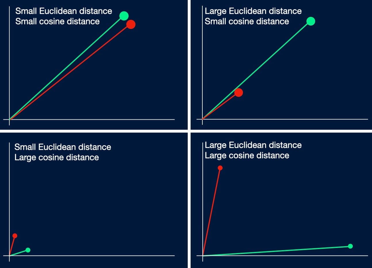
There are many ways of measuring the distance between vectors, and the choice of distance metric depends on the application. The typical choices are:
- Euclidean distance - straight line distance between points
- Cosine distance - the angle between two points
- Dot product - a projection of one vector onto another, which combines the magnitude and angle between two vectors (effectively a combination of Euclidean and Cosine distances)
- Manhattan distance - Distance when movement direction is constrained to be parallel to one axis at a time (i.e. no diagonal lines, as if following roads in the Manhattan grid system)
Euclidean distance is best for applications in which exact matching is important, like pixel values when comparing two images, while cosine distance is better for sentiment analysis, where very different combinations of letters and words can encode similar sentiments. Deciding on a distance metric requires an understanding of the data domain as well as the underlying problem, and since different metrics can yield very different answers to whether a pair of points are close or distant, this choice can make a lot of difference to the model's performance.
Vector Search
Vector search methods are ways of finding the closest match in a vector database to some input vector, e.g. the vector embedded query passed to our RAG model. This is a reasonably commonplace operation to perform with vector data, and standard k-nearest-neighbours (KNN) methods may be applied to find the relevant pieces of data. However, in application the retrieval architecture in a RAG will need to be able to return a result in a constrained timeframe of a few seconds, or maybe a few minutes for particularly patient users or complicated queries. If the vector database is large, perhaps holding millions of embedded data chunks, then finding the KNN can become prohibitively time-consuming.
Fortunately, for large databases, it is sufficient to return the approximate nearest neighbours (ANN) instead of the literal closest matches. While imperfect, enough context and information can generally be gleaned from this approach to answer the input query, and performance time at scale is much better.
A major ANN method in RAG is the hierarchical navigable small worlds method (HNSW), which arranges vectors as nodes on layers of connected graphs. Higher layers contain smaller subsets of the data set to be searched, and if a node is present on layer m, then it will be present on all layers lower than m. Searching begins on the top layer, with the search moving from node-to-node to minimise a distance metric between the node and the input query vector. If a closer match cannot be found on the current layer, it drops to the layer below and keeps going, until the closest match on the bottom level is reached.
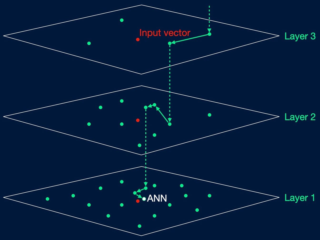
A full treatment of HNSW is worthy of its own post, and there are other approximate nearest neighbour search methods which can be applicable. Ultimately, the vector search step needs only to return a large enough number of sufficiently close matching results for the LLM, i.e. the generative model, to construct a meaningful and accurate answer.
Vector Databases
Vector databases are databases designed and optimised to handle vector data, as opposed to the tabular data stored by traditional relational databases. They provide efficient storage, indexing and querying mechanisms, optimised for high-dimensional and variable-length vectors, and thereby allow for flexible data storage and retrieval. Many vector databases are designed to scale horizontally, allowing for efficient distributed storage and querying across multiple nodes or clusters, and use techniques such as k-d trees, ball tres or locality-sensitive hashing to enable fast and efficient search operations.
Of particular use is the ability to associate metadata with each vector. For RAG applications, this allows a linkage between the raw, human-readable tokens of a text corpus to the abstract vector representation of a data chunk. This is of great utility in helping to debug and optimise a model, by letting the user interpret which results were found to be similar to an input vector and where the information for the returned query came from.
At the heart of RAG, vector databases can be thought of as a long term memory on top of a LLM, avoiding the need to retrain a model or rerun a dataset through a model before making a query.
LLM Interface Framework
With the vector database in place and populated, it’s necessary to have some way of interfacing it with a LLM, so that queries can be passed in and context can be returned. Two such interfacing frameworks currently available for use are LangChain and LlamaIndex, and either can be used to create a RAG model from a vector database and a LLM. Both are extensively documented by their developers and widely used in the AI community.
Platforms
Since RAG models lean heavily on the use of a vector database to enable their retrieval stage, platforms which support vector databases and enable vector search methods are required for deployment.
Existing solutions are available in the form of MongoDB’s Atlas with Atlas Vector Search and Pinecone’s Pinecone Vector Database with Vector Search, and open-source options such as Weaviate. Others are close to market, such as Oracle’s AI Vector Search, which will be included in a future update to Oracle Database 23c.
Benefits and Limitations of RAG
RAG offers a lot of potential improvement over purely generative models, at the cost of additional model complexity, up-front work and infrastructure. To help clarify this, we’ve summarised the main benefits and limitations of RAG models below.
Benefits of RAG
1. Reduced Hallucinations and Staleness
The vector database for retrieval can be kept up-to-date and made more complete than the stale training set of a pure generative model, leading to fewer hallucinations and decreasing the need to re-train the model.
2. Contextual Consistency
By retrieving data from a curated and maintained source database only, RAG helps to ensure that the output is contextually relevant and consistent with the input. The generative model will be focused on the data which answer the question, and not on the potentially irrelevant data on which it was trained.
3. Improved Accuracy
Similarly to the above, by grabbing data from a managed database of reliable information, the accuracy of responses is increased versus a pre-trained model alone.
4. Controllability
Using an appropriate retrieval database to provide ground truth to the generative model, and excluding any other sources, allows developers to control the scope of generated responses to the set of reliable, relevant and safe data.
5. Privacy
Rather than training an LLM on private data, it is instead possible to train an LLM generically and then point it towards private or proprietary data in a vector database as the context for a query. The data source acts as the LLM’s memory, and the model will not learn personally identifying or proprietary information.
6. Reduced Generation Bias
Retrieved context mitigates some of the generation biases observed in pure generative models, since biases from the training set will be superseded by the context from the vector database. While this does not prevent replication of biases which are extant in the vector database, it gives developers control over sources of bias, such that they can be corrected.
Limitations of RAG
1. Complexity
Joining two diverse models, a retrieval model and a generative model, is naturally going to increase the complexity over using a LLM alone. This means that more compute power is required and debugging is more complicated.
2. Data Preparation
As with any ML model, the RAG model requires clean, non-redundant and accurate data on which to base its answers. It then requires an effective chunking strategy to achieve the required efficiency and accuracy, and appropriate embedding to represent the data.
3. Prompt Engineering
Despite the capacity to search for relevant information, questions still need to be asked in the right way to yield a good answer. This can include a need to specify that only information in the retrieved context should be used to answer, and an effective wording of the search criteria.
4. Performance
The two-step process of searching followed by generation increases the real-time latency experienced from asking a question to receiving an answer, compared to using a generative model alone. This leads to a necessary trade-off between depth-of-search in the retrieval stage and overall response time.
Summary
That was a quick tour of RAG, covering the core concepts, the underlying technologies, and some of the options available for deploying a RAG model today. At its heart, RAG is a way of focusing a pre-trained generative model on relevant or private data without the risk of private data leakage, and with robustness against hallucinations, at the cost of a little complexity and infrastructure. As with any AI or ML architecture, it’s not a one-size-fits-all solution, nor is it a cure-all for the limitations of generative AI (for instance, the ethical problems of generative AI (e.g. a base LLM) being trained on copyrighted works), but it represents a major step forwards over purely generative models, and can be utilised for powerful time savings and efficiency gains.