Hyperion Essbase 11.1.1.2 – Varying Attributes
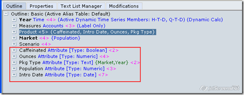
Another excellent feature that was introduced as part of the EPM 11 release was the support for varying attributes. Varying attributes help in providing different perspectives of multiple attributes of a dimension over time. One can visualize this as SCD 2 in a relational world. For example, lets take the Sample –> Basic cube and look at the various attributes that have been defined.
As you see, this cube has 5 different attributes defined on Product and Market dimensions. As of 9.3.1 release of Essbase one can have only static attributes defined. If varying attributes had to be defined, they had to be modeled as separate individual dimensions. Static attributes are those attributes that remain constant for a specific member. For example, lets assume that a product X has a static weight of Y ounces when it was introduced. If the manufacturing company decides to repackage the product X with a weight of Z ounces, then as of 9.3.1 release all the sales data mapped to Y ounces would switch over to Z ounces(similar to SCD-1 in a relational DW world). But in most cases, we want to see the sales data corresponding to their weights so that one can analyze the sales drop or increase due to the new product packaging. This is called as varying attributes over time. Sometimes, the same product X can be packaged with Y and Z ounces depending on Market. In this case, the weight varies over Time as well as Market.
With the advent of EPM 11.1.1.0, one can enable tracking of metrics over varying attributes as well. In the above outline, lets take the example of Pkg Type attribute. This has 2 values
- Bottle
- Can
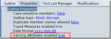
This packaging can vary for products across multiple Markets. Also the packaging can vary for a product in a specific market over time. To enable varying attributes, one would have to first enable this feature while creating an outline or later.
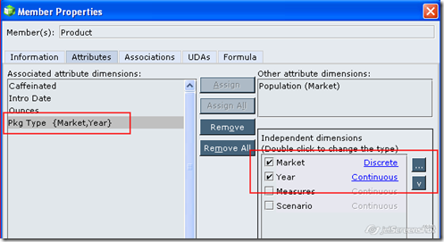
In order enable the attribute Pkg Type on the product dimension, one would have to choose the attribute and the set of independent dimensions. Independent dimensions are those dimensions over which the attribute varies like Market and Time.
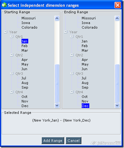
Continuous dimensions(in the screenshot above) are typically those dimensions like Time where there is a chronological order and where we can specify a range. After this has been enabled, while setting the attribute for each product, the Market and Time would have to be chosen as well. For continuous attributes, one can specify a range.
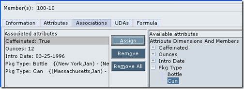
For each product set the Time range over which it is planned to be sold and also the market. In the above example, the product 100-10 is sold in New York Market from Jan till Dec in Bottle Type and in the Massachusetts Market from Jan to Dec in Can type. The same kind of association would have to be done for each and every Market for the corresponding Pkg Type.
The above basically provides a relational visualization in a multi-dimensional cube. This also provides analysis of data in multiple perspectives. For example, we might be needing a report wherein we would like to analyze the sales for the list of products that were sold as Bottles in New York from Jan-Dec with a perspective of the attribute setting that we had in July. These kind of queries can be answered pretty easily by Varying attributes. In a future blog entry we shall see how these varying attributes can be leveraged from BI EE. As of the current release in BI EE, one can only use the default query context/perspective. One cannot alter the perspectives due to the limitation of modifying certain parts of the MDX query in BI EE. Having said that, it is possible to leverage the varying attributes using the default perspective. I will cover this in the coming weeks.
