Spatial Analytics Made Easy: Oracle Spatial Studio

Oracle Spatial Studio: The new analytical tool to perform spatial analysis on a intuitive visual GUI

Francesco Tisiot

Jul 26, 2019 • 12 min read

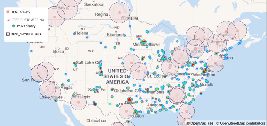
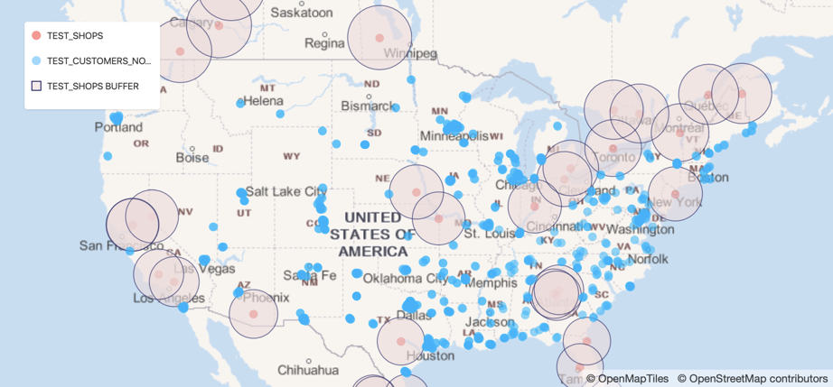
Let's say we need to understand where our company needs to open a new shop. Most of the time the decision is driven by gut feeling and some knowledge of the market and client base, but what if we could have visual insights about where are the high density zones with customers not covered by a shop nearby like in the map below?

Well... welcome Oracle Spatial Studio!

Spatial Studio is Oracle's new tool for creating spatial analytics with a visual GUI. It uses Oracle Spatial database functions in the backen d exposed with an interface in line with the Oracle Analytics Cloud one. Let's see how it works!

QuickStart Installation

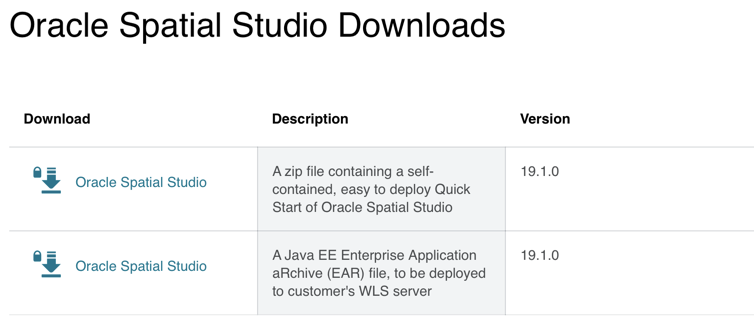
First of all we need to download Spatial Studio from the Oracle web page, for this initial test I downloaded the "Quick Start", a self contained version pre-deployed in a lightweight application server. For more robust applications you may want to download the EAR file deployable in Weblogic.

Once downloaded and unzipped the file, we just need to verify we have a Java JDK 8 (update 181 or higher) under the hood and we can immediately start Oracle Spatial Studio with the ./start.sh command.

The command will start the service on the local machine that can be accessed at https://localhost:4040/spatialstudio. By default Oracle Spatial Studio Quickstart uses HTTPS protocol with self-signed certificates, thus the first time you access the URL you will need to add a security exception in your browser. The configurations such as port, JVM parameters, host and HTTP/HTTPS protocol can be changed in the conf/server.json file.

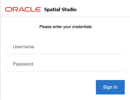
We can then login with the default credentials admin/welcome1

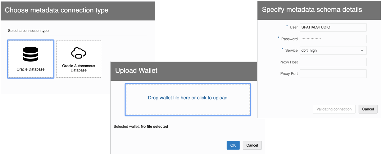
The first step in the Spatial Studio setup is the definition of the metadata connection type. This needs to point to an Oracle database with the spatial option. For my example I initially used an Oracle Autonomous Data Warehouse, for which I had to drop the wallet and specify the schema details.

Once logged in, the layout and working flows are very similar to Oracle Analytics Cloud making the transition between the two very easy (more details on this later on). In the left menu we can access, like in OAC, Projects (visualizations), Data, Jobs and the Console.

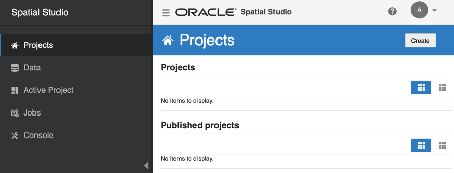
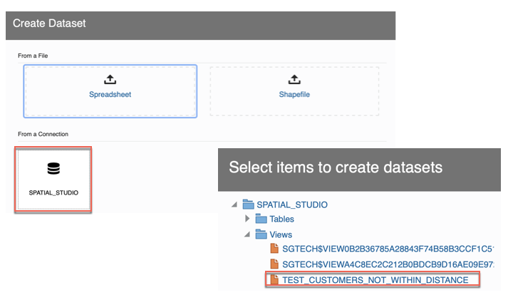
In order to do Spatial Analysis we need to start from a Dataset, this can be existing tables or views, or we can upload local files. To create a Dataset, click on Create and Dataset

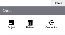
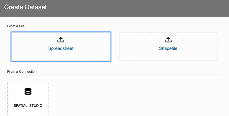
We have then three options:

Upload a Spreadsheet containing spatial information (e.g. Addresses, Postcodes, Regions, Cities etc)
Upload a Shapefile containing geometric locations and associated attributes.
Use spatial data from one of the existing connections, this can point to any connection containing spatial information (e.g. a table in a database containing customer addresses)

Sample Dataset with Mockaroo

I used Mockaroo, a realistic data generator service, to create two excel files: one containing customers with related locations and a second one with shops and related latitude and longitude. All I had to do was to select which fields I wanted to include in my file and the related datatype.

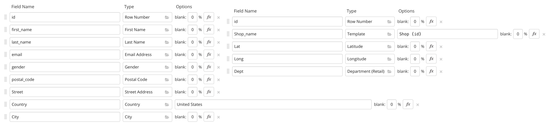
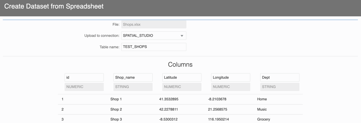
For example, the list of shop dataset contained the following columns:

Id: as row number
Shop Name: as concatenation of Shop and the Id
Lat: Latitude
Long: Longitude
Dept: the Department (e.g. Grocery, Books, Health&Beauty)

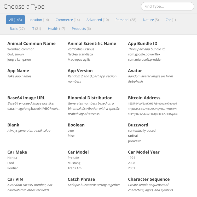
Mockaroo offers a perfect service and has a free tier of datasets with less than 1000 rows which can be useful for demo purposes. For each column defined, you can select between a good variety of column types. You can also define your own type using regular expressions!

Adding the Datasets to Oracle Spatial Studio

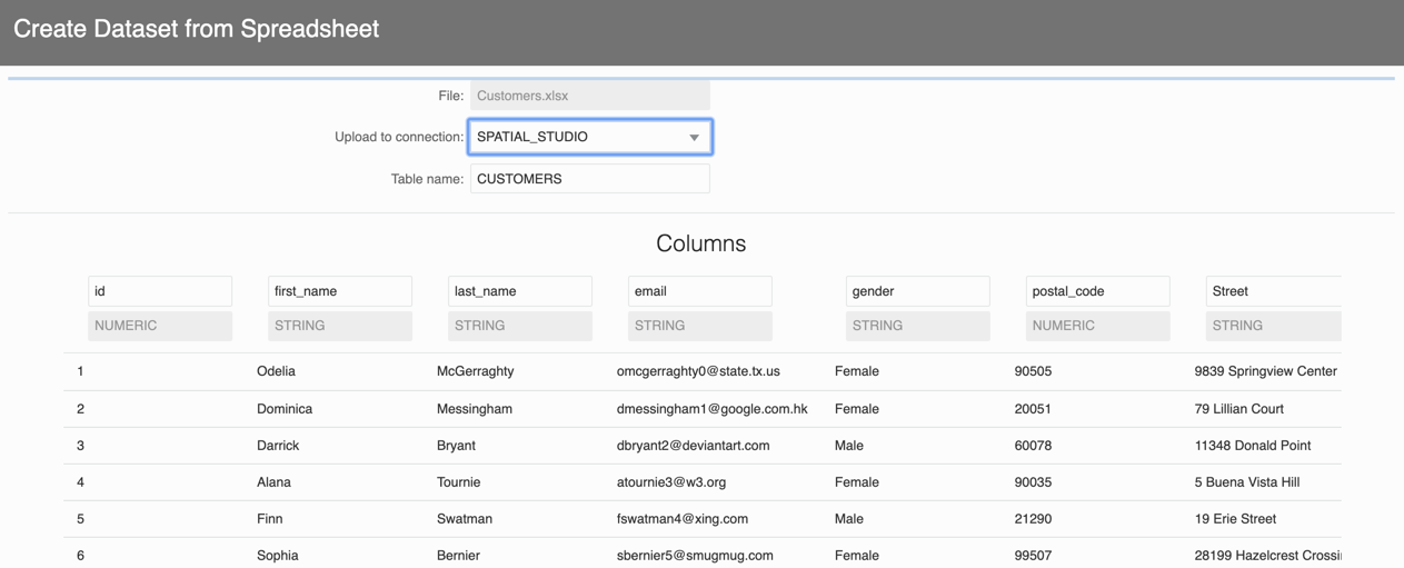
Once we have the two datasources in Excel format, it's time to start playing with Spatial Studio. We first need to upload the datasets, we can do it via Create and Dataset. Starting with the Customer.xlsx one. Once selected the file to upload Spatial Studio provides (as OAC) an overview of the dataset together with options to change configurations like dataset name, target destination (metadata database) and column names.

Once modified the table name to TEST_CUSTOMERS and clicked on Submit Spatial Studio starts inserting all the rows into the SPATIAL_STUDIO connection with a routine that could take seconds or minutes depending on the dataset volume. When the upload routine finishes I can see the TEST_CUSTOMERS table appearing in the list of datasets.

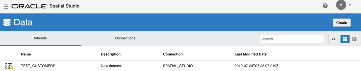
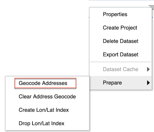
We can immediately see the yellow warning sign next to the dataset name, it's due to the fact that we have a dataset with no geo-coded information, we can solve this problem by clicking on the option button and then Prepare and Geocode Addresses

Oracle Spatial Studio will suggest, based on the column content, some geo-type matching e.g. City Name, Country and Postal Code. We can use the defaults or modify them if we feel they are wrong.

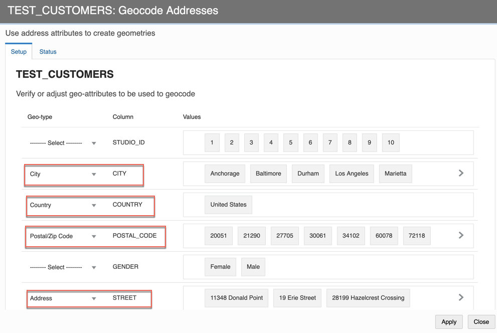
Once clicked on Apply the geocoding job starts.

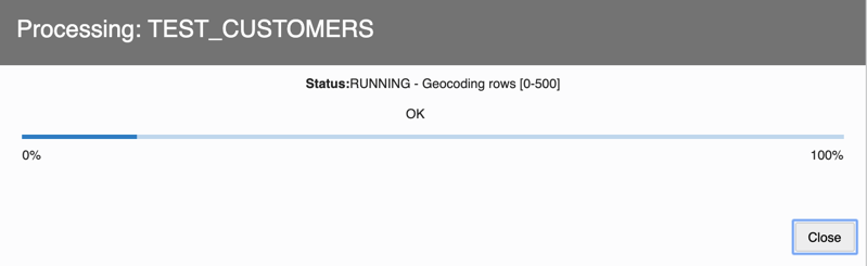
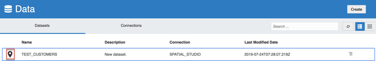
Once the job ends, we can see the location icon next to our dataset name

We can do the same for the Shops.xlsx dataset, starting by uploading it and store it as TEST_SHOPS dataset.

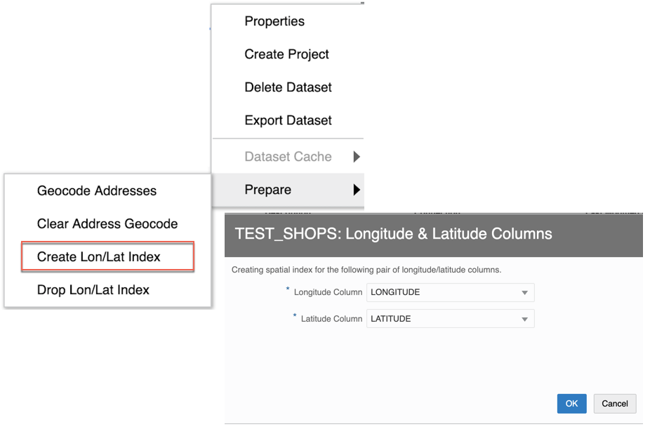
Once the dataset is uploaded I can geo-locate the information based on the Latitude and Longitude, I can click on the option button and the selecting Prepare and Create Lon/Lat Index. Then I'll need to assign the Longitude and Latitude column correctly and click on Ok.

Spatial Analytics

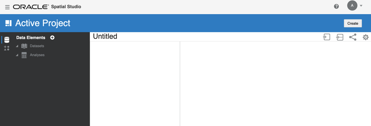
Now it's time to do some Spatial Analysis so I can click on Create and Project and I'll face an empty canvas by default

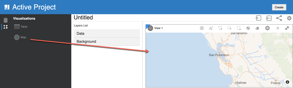
The first step is to add a Map, I can do that by selecting the visualizations menu and then dragging the map to the canvas.

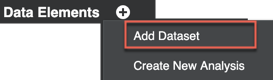
Next step is to add some data by clicking on Data Elements and then Add Dataset

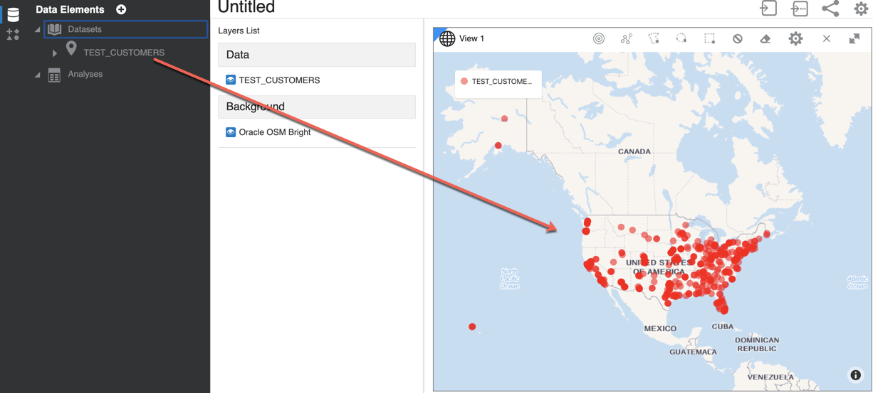
I select the TEST_CUSTOMERS dataset and add it to the project, then I need to drag it on top of the map to visualize my customer data.

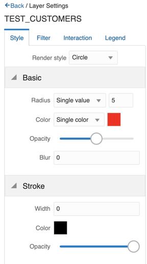
Oracle Spatial Studio Offers several options to change the data visualizations like color, opacity, blur etc.

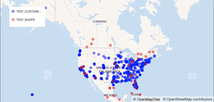
Now I can add the TEST_SHOPS dataset and visualize it on the map with the same set of steps followed before.

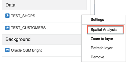
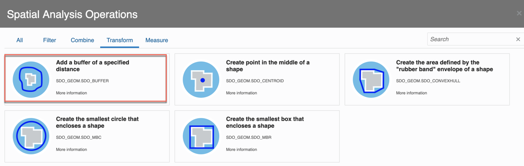
It's finally time for spatial analysis! Let's say, as per initial example, that I want to know which of my customers doesn't have any shops in the nearest 200km. In order to achieve that I need to first create buffer areas of 200km around the shops, by selecting the TEST_SHOPS datasource and then clicking on the Spatial Analysis.

This will open a popup window listing a good number of spatial analysis, by clicking on the Transform tab I can see the Add a buffer of a specified distance option.

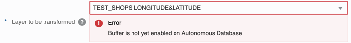
Unfortunately the buffer function is not available in ADW at the moment.

I had to rely on an Oracle Database Cloud Service 18c Enterprise Edition - High Performance (which includes the Spatial option) to continue for my metadata storage and processing. Few Takeaways:

Select 18c (or anything above 12.2): I hit an issue ORA-00972: identifier is too long when importing the data in a 12.1 Database, which (thanks StackOverflow) is fixed as of 12.2.
High Performance: This includes the Spatial Option

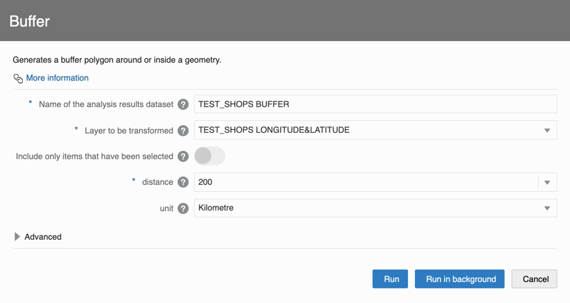
Once I used the DBCS as metadata store, I can finally use the buffer function and set the parameter of 200km around the shops.

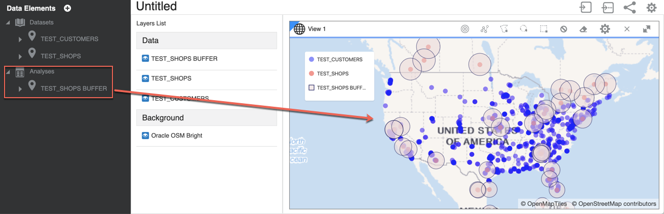
The TEST_SHOPS_BUFFER is now visible under Analysis and can be added on top of the Map correctly showing the 200km buffer zone.

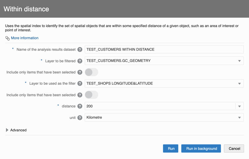
I can understand which customers have a shop in the nearest 200k by creating an analysis and select the option "Return shapes within a specified distance of another"

In the parameters I can select the TEST_CUSTOMERS as Layer to be filtered, the TEST_SHOPS as the Layer to be used as filter and the 200Km as distance.

I can then visualize the result by adding the TEST_CUSTOMERS_WITHIN_DISTANCE layer in the map.

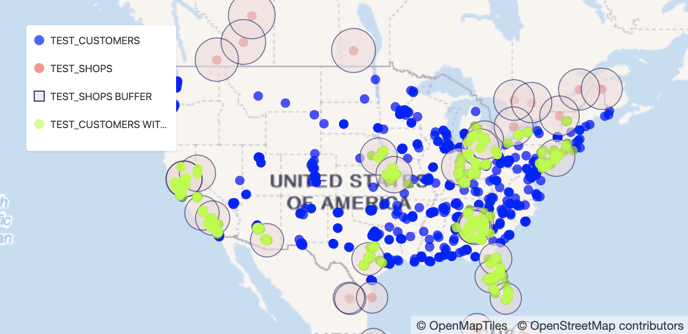
TEST_CUSTOMERS_WITHIN_DISTANCE contains the customers already "covered" by a shop in the 200km range, what I may want to do now is remove them from my list of customers in order to do analysis on the remaining ones, how can I do that? Unfortunately in the first Spatial Studio version there is no visual way of doing DATASET_A MINUS DATASET_B but, hey, it's just the first incarnation and we can expect that type of functions and many others to be available in future releases!

The following paragraph is an in-depth analysis in the database of functions that will probably be exposed in Spatial Studio's future version, so if not interested, progress directly to the section named "Progressing in the Spatial Analysis".

A Look in the Database

Since we want to achieve our goal of getting the customers not covered by a shop now, we need to look a bit deeper where the data is stored: in the database. This gives us two opportunities: check how Spatial Studio works under the covers and freely use SQL to achieve our goals (DATASET_A MINUS DATASET_B).

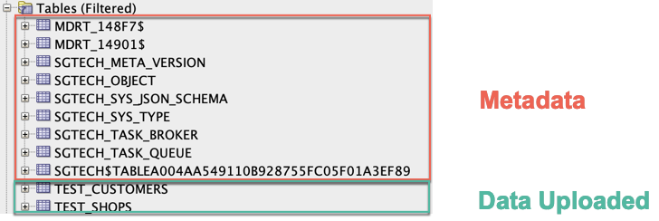
First let's have a look at the tables created by Spatial Studio: we can see some metadata tables used by studio as well as the database representation of our two excel files TEST_CUSTOMERS and TEST_SHOPS.

Looking in depth at the metadata we can also see a table named SGTECH$TABLE followed by an ID. That table collects the information regarding the geo-coding job we executed against our customers dataset which were located starting from zip-codes and addresses. We can associate the table to the TEST_CUSTOMERS dataset with the following query against the SGTECH_OBJECTS metadata table.

SELECT NAME, 
  JSON_VALUE(data, '$.gcHelperTableName') DATASET  
FROM SGTECH_OBJECT 
WHERE OBJECTTYPE='dataset'
AND NAME='TEST_CUSTOMERS';

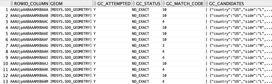
The SGTECH$TABLEA004AA549110B928755FC05F01A3EF89 table contains, as expected, a row for each customer in the dataset, together with the related geometry if the geo-coding was successful and some metadata flags like GC_ATTEMPTED, GC_STATUS and GC_MATCH_CODE stating the accuracy of the geo-coding match.

What about all the analysis like the buffer and the customers within distance? For each analysis Spatial Studio creates a separate view with the SGTECH$VIEW prefix followed by an ID.

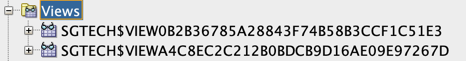
To understand which view is referring to which analysis we need to query the metadata table SGTECH_OBJECTS with a query like

SELECT NAME, 
  JSON_VALUE(data, '$.tableName') DATASET  
FROM SGTECH_OBJECT 
WHERE OBJECTTYPE='dataset'

With the following result

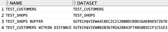
We know then that the TEST_CUSTOMERS_WITHIN_DISTANCE can be accessed by the view SGTECH$VIEW0B2B36785A28843F74B58B3CCF1C51E3 and when checking its SQL we can clearly see that it executes the SDO_WITHIN_DISTANCE function using the TEST_CUSTOMERS.GC_GEOMETRY, the TEST_SHOPS columns LONGITUDE and LATITUDE and the distance=200 unit=KILOMETER parameters we set in the front-end.

CREATE OR replace force editionable view "SPATIAL_STUDIO"."SGTECH$VIEW0B2B36785A28843F74B58B3CCF1C51E3"
SELECT
    ...
FROM
    "TEST_CUSTOMERS"   "t1",
    "TEST_SHOPS"       "t2"
WHERE
    sdo_within_distance("t1"."GC_GEOMETRY",
    spatial_studio.sgtech_ptf("t2"."LONGITUDE", "t2"."LATITUDE"), 
    'distance=200 unit=KILOMETER'
    ) = 'TRUE';

Ok, we now understood which view contains the data, thus we can create a new view containing only the customers which are not within the 200km distance with

CREATE VIEW TEST_CUSTOMERS_NOT_WITHIN_DISTANCE AS
SELECT
    t1.id            AS id,
    t1.first_name    AS first_name,
    t1.last_name     AS last_name,
    t1.email         AS email,
    t1.gender        AS gender,
    t1.postal_code   AS postal_code,
    t1.street        AS street,
    t1.country       AS COUNTRY,
    t1.city          AS city,
    t1.studio_id     AS studio_id,
    t1.gc_geometry   AS gc_geometry
FROM
    test_customers t1
WHERE
    id NOT IN (
        SELECT
            id
        FROM
            spatial_studio.sgtech$view0b2b36785a28843f74b58b3ccf1c51e3
    );

Progressing in the Spatial Analysis

In the previous paragraph we created a view in the database named TEST_CUSTOMERS_NOT_WITHIN_DISTANCE containing the customer without a shop in a 200km radius. We can now import it into Spatial Studio by creating a new dataset, selecting the connection to the database (in our case named SPATIAL_STUDIO) as source and then the newly created TEST_CUSTOMERS_NOT_WITHIN_DISTANCE view.

The dataset is added, but it has a yellow warning icon next to it

Spatial Studio requests us to define a primary key, we can do that by accessing the properties of the dataset, select the Columns tab, choosing which column acts as primary key and validate it. After this step I can visualize this customer in a map.

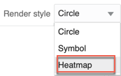
What's next? Well If I want to open a new shop, I may want to do that where there is a concentration of customers, which is easily visualizable with Spatial Studio by changing the Render Style to Heatmap.

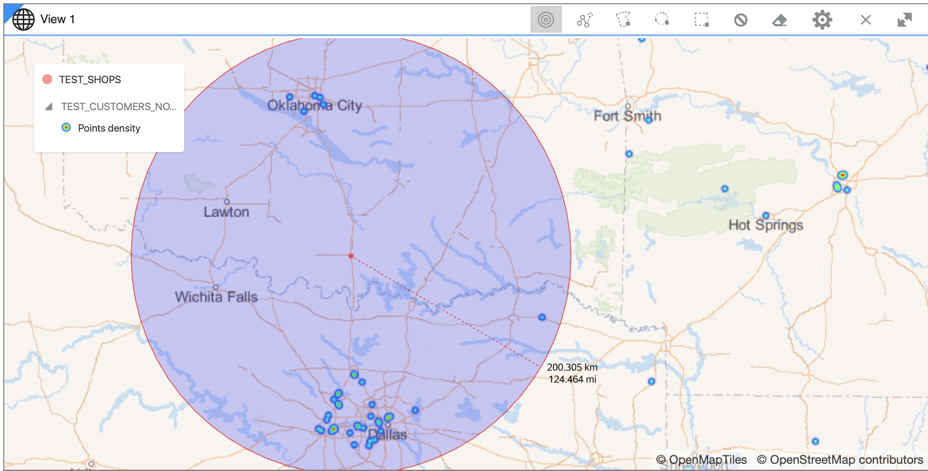
With the following output

We can clearly see some major concentrations around Dallas, Washington and Minneapolis. Focusing more on Dallas, Spatial Studio also offers the option to simulate a new shop in the map and calculate the 200km buffer around it. I can clearly see that adding a shop halfway between Oklahoma City and Dallas would allow me to cover both clients within the 200km radius.

Please remember that this is a purely demonstrative analysis, and some of the choices, like the 200km buffer are expressly simplistic. Other factors could come into play when choosing a shop location like the revenue generated by some customers. And here it comes the second beauty of Oracle Spatial Studio, we can export datasets as GeoJSON or CSV and include them in Data Visualization.

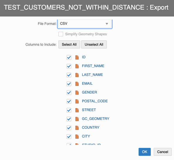
For example I can export the data of TEST_CUSTOMERS_NOT_WITHIN_DISTANCE from Spatial Studio and include then in a Data Visualization Project blending them with the Sales related to the same customers.

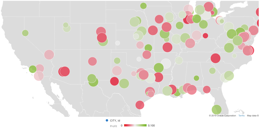
I can now focus not only on the customer's position but also on other metrics like Profit or Sales Amount that I may have in other datasets. For another example of Oracle Spatial Studio and Data Visualization interoperability check out this video from Oracle Analytics Senior Director Philippe Lions.

Conclusions

Spatial analytics made easy: this is the focus of Oracle Spatial Studio. Before spatial queries were locked down at database level with limited access from an analyst point of view. Now we have a visual tool with a simple GUI (in line with OAC) that easily enables spatial queries for everybody!

But this is only the first part of the story: the combination of capabilities achievable when mixing Oracle Spatial Studio and Oracle Analytics Cloud takes any type of analytics to the next level!