Bitmap Indexes Redux
I was running a data warehousing training event for a client recently, and in one of the sessions we looked at bitmap indexes and bitmap join indexes. Whilst the session went OK I remember thinking to myself at the end, "you know what, there's a fair bit about bitmap indexes I'm not too clear on", and so I made a mental note after the session to take a closer look at how they work.
Of course bitmap indexes, and indexes in general, are a subject that people like Richard Foote and Jonathan Lewis have covered very well in the past and there are number of good article on the internet that explain how the feature works. In particular three articles by Jonathan, on bitmap indexes, bitmap star transformations and bitmap join indexes, are about the closest I've seen to a definitive introduction to the subject, whereas this article by Vivek Sharma compares bitmap indexes to b- tree indexes in the context of decision support with some useful examples of test cases to illustrate the differences. There's also a good article on Wikipedia that sets out a generic background to bitmap indexes, which of course are used across the database industry and aren't just an Oracle feature. Looking through these articles was certainly useful in filling in some of the gaps in my knowledge, and in particular confirmed the basic understanding that I had around the subject.
Bitmap indexes differ from the more common b-tree indexes in that they use bit arrays (also known as "bitmaps") to indicate whether a particular row in a table contains a particular column value. To take an example, you might have a table of customer details, and you have a column called "hair colour". A bitmap index on this column would logically store the index data in the following way:
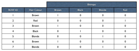
- A set of flags
- A lock byte
- The indexed value ("Red Hair", for example, or "Big Feet")
- A pair of row IDs, and
- A stream of bits
The lock byte is used to determine whether this particular part of the index is locked, because of some DML happening to the underlying table. The pair of row IDs designates the portion of the table that this index leaf block covers (back in the 9i days, Jonathan reckons this range can cover up to 24,000 rows, this may have changed with more recent releases), whilst the stream of bits tells Oracle whether a particular row ID contains the indexed value in question. Presumably then some sort of compression algorithm is applied and, depending on the number of distinct values that are being indexed and the distribution of the data, the index is then stored taking up potentially far less space than a regular b- tree index.
So the general thinking here is that bitmap indexes are particularly suited to decision support applications as they
(a) can be easily combined using bit-wise operations to filter data based on multiple criteria
(b) their high compression ratios mean that they can take up less space than comparable b- tree indexes
(c) they can be quick to create, meaning you can create more of them in a given ETL window or your ETL process can take less time, and
(d) if you are using Oracle, you can use additional features such as bitmap star transformations to rapidly return data from your data warehouse.
Now there are a lot of claims, myths and ideas out there about bitmap indexes which are partly explained by the fact that it's often it's difficult to test them under the right conditions (multiple concurrent users, for example, or with big enough data sets) and the characteristics of the feature have changed over time (the effect of multiple updates onto bitmap-indexed columns has become less pronounced since the advent of 10g, with these two blog postings (here, and here) being good examples of where people can end up drawing the wrong conclusions.
That said though, looking back at the session I ran, in hindsight what it lacked were some basic examples of bitmap index creation, with some tests afterwards to compare their build time, size and query performance compared to regular b-tree indexes. I'm also curious to see what extra benefit is gained by using bitmap join indexes both in comparison to regular bitmap indexes and compared to what seems to me to be a similar thing - creating join-only materialized views (though I could be wrong here). Given this, I took the SH Sales History data set and started to knock up some examples. Now bear with me here as this is still only a very limited example, I'm also happy for anyone who knows more about this (Pete? Richard? Stuart?) to chip in and point out if I've drawn the wrong conclusion.
To start off then, I'm going to take two copies of the SH.CUSTOMERS table, and load the table data back into the tables a couple of times to increase the table row counts, otherwise most of the tests I do will return data too quickly. The version I'm using of Oracle is 11.1.0.6 on Windows XP SP2, running on a VMWare Fusion virtual machine with 1.25GB of RAM and 1 processor enabled.
SQL> select count(*) from customers_copy_btree;

COUNT(*)
----------
1776000

SQL> select count(*) from customers_copy_bitmap;

COUNT(*)
----------
1776000
OK, so both CUSTOMER table copies have now got around 1.7M rows within them. The SH schema from which they are sourced is a star schema, so the CUSTOMERS table has lots of "attribute" columns that I can index and then filter on.
SQL> select count(distinct cust_gender) from customers_copy_bitmap;

COUNT(DISTINCTCUST_GENDER)
--------------------------
2

SQL> select count(distinct cust_year_of_birth) from customers_copy_bitmap;

COUNT(DISTINCTCUST_YEAR_OF_BIRTH)
---------------------------------
75

SQL> select count(distinct cust_last_name) from customers_copy_bitmap;

COUNT(DISTINCTCUST_LAST_NAME)
-----------------------------
908

SQL> select count(distinct cust_street_address) from customers_copy_bitmap;

COUNT(DISTINCTCUST_STREET_ADDRESS)
----------------------------------
50945
So looking at those distinct row counts, the table's attributes range from 2 distinct values (gender) through 75 (year of birth) through to 50,945 for street addresses. That should give us a range of different column cardinalities to test.
SQL> set timing on

SQL> create index cus_gender_btree_idx on customers_copy_btree(cust_gender);

Index created.

Elapsed: 00:00:34.01

SQL> create index cus_yob_btree_idx on customers_copy_btree(cust_year_of_birth);

Index created.

Elapsed: 00:00:37.12

SQL> create index cus_lname_btree_idx on customers_copy_btree(cust_last_name);

Index created.

Elapsed: 00:00:29.25

SQL> create index cus_adr_btree_idx on customers_copy_btree(cust_street_address);

Index created.

Elapsed: 00:00:46.43
Creating b-tree indexes on a selection of columns comes in at a total of 34+37+29+46 = 2 mins 26 seconds. How long to comparable bitmap indexes take to create?
SQL> create bitmap index cus_gender_bix on customers_copy_bitmap(cust_gender);

Index created.

Elapsed: 00:00:36.11

SQL> create bitmap index cus_yob_bix on customers_copy_bitmap(cust_year_of_birth);

Index created.

Elapsed: 00:00:10.57

SQL> create bitmap index cus_lname_bix on customers_copy_bitmap(cust_last_name);

Index created.

Elapsed: 00:00:13.92

SQL> create bitmap index cus_adr_bix on customers_copy_bitmap(cust_street_address);

Index created.

Elapsed: 00:00:10.87
So to create the bitmap indexes, the total time was 36+10+14+10 = 1 min 10 seconds, about half the time of the b-tree indexes. I then gather statistics on the tables and indexes and then run a query to determine the table and index sizes.
SQL> select segment_name
2  ,	    bytes/1024/1024 "Size in MB"
3  from   user_segments
4  where  segment_name like 'CUSTOMERS_COPY%';

SEGMENT_NAME                             Size in MB
---------------------------------------- ----------
CUSTOMERS_COPY_BITMAP                           368
CUSTOMERS_COPY_BTREE                            368

SQL> select segment_name
2  ,	    bytes/1024/1024 "Size in MB"
3  from   user_segments
4  where  segment_name like '%_IDX';

SEGMENT_NAME                             Size in MB
---------------------------------------- ----------
CUS_ADR_BTREE_IDX                                72
CUS_GENDER_BTREE_IDX                             26
CUS_LNAME_BTREE_IDX                              36
CUS_YOB_BTREE_IDX                                30

SQL> select segment_name
2  ,	    bytes/1024/1024 "Size in MB"
3  from   user_segments
4  where  segment_name like '%_BIX';

SEGMENT_NAME                             Size in MB
---------------------------------------- ----------
CUS_ADR_BIX                                      11
CUS_GENDER_BIX                                 .625
CUS_LNAME_BIX                                     3
CUS_YOB_BIX                                       5
The tables we're indexing are 368MB in size, and the b-tree indexes range from 72MB for the high-cardinality address index, through to 30MB for the low-cardinality gender index. The bitmap indexes, though, are around six times smaller, going from 11MB for the address index through to just over half a MB for the gender index. So they're certainly smaller, at least for this dataset's data distribution, and as we saw before, they take less time to prepare.
How about some queries then, how do the explain plans look for simple queries using these columns as filters? Let's try filtering on year of birth, which had 75 different values in our test data.
SQL> set lines 200
SQL> set autotrace traceonly
SQL> select *
  2  from   customers_copy_btree
  3  where  cust_year_of_birth = 1967;

30592 rows selected.

Execution Plan
----------------------------------------------------------
Plan hash value: 2533345702
------------------------------------------------------------------------------------------
| Id  | Operation         | Name                 | Rows  | Bytes | Cost (%CPU)| Time     |
------------------------------------------------------------------------------------------
|   0 | SELECT STATEMENT  |                      | 30592 |  5526K| 12728   (1)| 00:02:33 |
|*  1 |  TABLE ACCESS FULL| CUSTOMERS_COPY_BTREE | 30592 |  5526K| 12728   (1)| 00:02:33 |
------------------------------------------------------------------------------------------

Predicate Information (identified by operation id):
---------------------------------------------------

   1 - filter("CUST_YEAR_OF_BIRTH"=1967)

Statistics
----------------------------------------------------------
          1  recursive calls
          0  db block gets
      48332  consistent gets
      46337  physical reads
          0  redo size
    4711189  bytes sent via SQL*Net to client
      22845  bytes received via SQL*Net from client
       2041  SQL*Net roundtrips to/from client
          0  sorts (memory)
          0  sorts (disk)
      30592  rows processed

SQL> select *
  2  from   customers_copy_bitmap
  3  where  cust_year_of_birth = 1967;

30592 rows selected.

Execution Plan
----------------------------------------------------------
Plan hash value: 3003431057

------------------------------------------------------------------------------------------------------
| Id  | Operation                    | Name                  | Rows  | Bytes | Cost (%CPU)| Time     |
------------------------------------------------------------------------------------------------------
|   0 | SELECT STATEMENT             |                       | 30592 |  5526K|  5652   (1)| 00:01:08 |
|   1 |  TABLE ACCESS BY INDEX ROWID | CUSTOMERS_COPY_BITMAP | 30592 |  5526K|  5652   (1)| 00:01:08 |
|   2 |   BITMAP CONVERSION TO ROWIDS|                       |       |       |            |          |
|*  3 |    BITMAP INDEX SINGLE VALUE | CUS_YOB_BIX           |       |       |            |          |
------------------------------------------------------------------------------------------------------

Predicate Information (identified by operation id):
---------------------------------------------------

   3 - access("CUST_YEAR_OF_BIRTH"=1967)

Statistics
----------------------------------------------------------
        170  recursive calls
          0  db block gets
      24427  consistent gets
      16164  physical reads
          0  redo size
    5975063  bytes sent via SQL*Net to client
      22845  bytes received via SQL*Net from client
       2041  SQL*Net roundtrips to/from client
          0  sorts (memory)
          0  sorts (disk)
      30592  rows processed
So in that example, Oracle actually used a full table scan for the b-tree indexed table, whilst the bitmap indexed one used an index lookup. The cost of the execution plan against the bitmap indexed table was the lowest out of the two. Now what about if we filter on several columns, this is where bitmap indexes surely come into their own?
SQL> select *
  2  from   customers_copy_bitmap
  3  where  cust_gender = 'M'
  4  and    cust_year_of_birth = 1980
  5  and    cust_last_name = 'SMITH';

no rows selected

Execution Plan
----------------------------------------------------------
Plan hash value: 2767299321

------------------------------------------------------------------------------------------------------
| Id  | Operation                    | Name                  | Rows  | Bytes | Cost (%CPU)| Time     |
------------------------------------------------------------------------------------------------------
|   0 | SELECT STATEMENT             |                       |    21 |  3885 |     8   (0)| 00:00:01 |
|   1 |  TABLE ACCESS BY INDEX ROWID | CUSTOMERS_COPY_BITMAP |    21 |  3885 |     8   (0)| 00:00:01 |
|   2 |   BITMAP CONVERSION TO ROWIDS|                       |       |       |            |          |
|   3 |    BITMAP AND                |                       |       |       |            |          |
|*  4 |     BITMAP INDEX SINGLE VALUE| CUS_LNAME_BIX         |       |       |            |          |
|*  5 |     BITMAP INDEX SINGLE VALUE| CUS_YOB_BIX           |       |       |            |          |
|*  6 |     BITMAP INDEX SINGLE VALUE| CUS_GENDER_BIX        |       |       |            |          |
------------------------------------------------------------------------------------------------------

Predicate Information (identified by operation id):
---------------------------------------------------
   4 - access("CUST_LAST_NAME"='SMITH')
   5 - access("CUST_YEAR_OF_BIRTH"=1980)
   6 - access("CUST_GENDER"='M')

Statistics
----------------------------------------------------------
          1  recursive calls
          0  db block gets
          2  consistent gets
          2  physical reads
          0  redo size
       1701  bytes sent via SQL*Net to client
        405  bytes received via SQL*Net from client
          1  SQL*Net roundtrips to/from client
          0  sorts (memory)
          0  sorts (disk)
          0  rows processed

SQL> select *
  2  from   customers_copy_btree
  3  where  cust_gender = 'M'
  4  and    cust_year_of_birth = 1980
  5  and    cust_last_name = 'SMITH';

no rows selected

Execution Plan

----------------------------------------------------------
Plan hash value: 2580896903

---------------------------------------------------------------------------------------------------------
| Id  | Operation                        | Name                 | Rows  | Bytes | Cost (%CPU)| Time     |
---------------------------------------------------------------------------------------------------------
|   0 | SELECT STATEMENT                 |                      |    21 |  3885 |    77   (2)| 00:00:01 |
|*  1 |  TABLE ACCESS BY INDEX ROWID     | CUSTOMERS_COPY_BTREE |    21 |  3885 |    77   (2)| 00:00:01 |
|   2 |   BITMAP CONVERSION TO ROWIDS    |                      |       |       |            |          |
|   3 |    BITMAP AND                    |                      |       |       |            |          |
|   4 |     BITMAP CONVERSION FROM ROWIDS|                      |       |       |            |          |
|*  5 |      INDEX RANGE SCAN            | CUS_LNAME_BTREE_IDX  |  1956 |       |     7   (0)| 00:00:01 |
|   6 |     BITMAP CONVERSION FROM ROWIDS|                      |       |       |            |          |
|*  7 |      INDEX RANGE SCAN            | CUS_YOB_BTREE_IDX    |  1956 |       |    62   (0)| 00:00:01 |
---------------------------------------------------------------------------------------------------------

Predicate Information (identified by operation id):
---------------------------------------------------
   1 - filter("CUST_GENDER"='M')
   5 - access("CUST_LAST_NAME"='SMITH')
   7 - access("CUST_YEAR_OF_BIRTH"=1980)

Statistics
----------------------------------------------------------
          1  recursive calls
          0  db block gets
          3  consistent gets
          2  physical reads
          0  redo size
       1701  bytes sent via SQL*Net to client
        405  bytes received via SQL*Net from client
          1  SQL*Net roundtrips to/from client
          0  sorts (memory)
          0  sorts (disk)
          0  rows processed
Interestingly, Oracle has converted the b-tree indexes into bitmap ones, when querying the b-tree indexed table, so that it can do a bitmap AND on the filter results, which I presume brings the performance of data warehouse b-tree queries closer to "native" bitmap ones (this, I think, has been a feature of the database since the 10g version at least). Even so, the cost of the bitmap query appears to be a lot less than the b-tree index one, and so far, the results are as you'd expect.
So what about the famous issue with bitmap indexes, the one where updates to the column that's indexed cause the index to grow in size, because the index loses compression? The fact this happens seems to be received wisdom, especially when updates are in the form of lots of little updates rather than a small amount of large updates, however people have mentioned that in recent versions, the effect is less pronounced. The other commonly held issue with updates against bitmap indexes is that they are slow, in comparison to tables with regular b-tree indexes, but this seems to be more of an issue when the updates are applied concurrently, due to portions of the indexed table (or perhaps portions of the indexed column) getting locked whilst the associated bitmap index is reconfigured. The concurrency test is tricky to perform when you've just got a single-user laptop, but what about the size issue, what if I applied a couple of hundred single-row updates to a bitmap indexed table and column using Oracle 11.1.0.6, would this increase the size of the index now?
SQL> create index test_cust_id_1_idx on customers_copy_btree (cust_id);

Index created.

SQL> create index test_cust_id_2_idx on customers_copy_bitmap (cust_id);

Index created.

SQL> set timing on

SQL> declare
  2  upd_cust_id number(5);
  3  cust_yob_value number(4);
  4  begin
  5    for i in 1 .. 500 loop
  6  	 upd_cust_id := dbms_random.value(1,55000);
  7  	 cust_yob_value := dbms_random.value(1900,2000);
  8  	 update customers_copy_btree
  9  	   set cust_year_of_birth = cust_yob_value
 10  	   where cust_id = upd_cust_id;
 11  	 commit;
 12    end loop;
 13  end;
 14  /

PL/SQL procedure successfully completed.

Elapsed: 00:03:15.67

SQL> declare
  2  upd_cust_id number(5);
  3  cust_yob_value number(4);
  4  begin
  5    for i in 1 .. 500 loop
  6  	 upd_cust_id := dbms_random.value(1,55000);
  7  	 cust_yob_value := dbms_random.value(1900,2000);
  8  	 update customers_copy_bitmap
  9  	   set cust_year_of_birth = cust_yob_value
 10  	   where cust_id = upd_cust_id;
 11  	 commit;
 12    end loop;
 13  end;
 14  /

PL/SQL procedure successfully completed.

Elapsed: 00:05:46.21

SQL> set timing off

SQL> select segment_name
  2  ,	    bytes/1024/1024 "Size in MB"
  3  from   user_segments
  4  where  segment_name in ('CUS_YOB_BTREE_IDX','CUS_YOB_BIX');

SEGMENT_NAME                             Size in MB
---------------------------------------- ----------
CUS_YOB_BIX                                       5
CUS_YOB_BTREE_IDX                                30
So the update to the bitmap indexed column took a fair bit longer than the b-tree indexed column, although as I said this should really be tested with lots of concurrent updates as this is where, I believe, the effect is most pronounced. When it comes to the size of the indexes though, they're more or less the same as before the updates took place, which seems to indicate that in this release, bitmap indexes don't grow is size so much when updates are applied. YMMV though.
Ok, so how about bitmap join indexes though? If we've got a fact table that we want to join to the dimension table, how much better performance do we get if we create bitmap join indexes on the fact table that join to the dimension key and dimension attribute values, compared to just standard bitmap indexes? To test this I took a copy of the SH.SALES and SH.CUSTOMER tables and created some example indexes.
SQL> select count(*) from customers_bijx_test_bitmap;

  COUNT(*)
----------
     55500

SQL> select count(*) from sales_bijx_test_bitmap;

  COUNT(*)
----------
  14701488

SQL> alter table customers_bijx_test_bitmap add constraint cust_bijx_test_bitmap_pk primary key (cust_id);

Table altered.

SQL> select count(*) from customers_bijx_test_bitjoin;

  COUNT(*)
----------
     55500

SQL> select count(*) from sales_bijx_test_bitjoin;

  COUNT(*)
----------
  14701488

SQL> alter table customers_bijx_test_bitjoin add constraint cust_bijx_test_bitjoin_pk primary key (cust_id);

SQL> set timing on

SQL> create bitmap index sales_bijx_test_bitmap_bix1 on sales_bijx_test_bitmap(cust_id);

Index created.

Elapsed: 00:00:33.43

SQL> create bitmap index cust_bijx_test_bitmap_bix1 on customers_bijx_test_bitmap(cust_last_name);

Index created.

Elapsed: 00:00:00.73

SQL> create bitmap index sales_bijx_test_bitjoin_bjx1 on sales_bijx_test_bitjoin(customers_bijx_test_bitjoin.cust_id)
  2  from sales_bijx_test_bitjoin, customers_bijx_test_bitjoin
  3  where sales_bijx_test_bitjoin.cust_id = customers_bijx_test_bitjoin.cust_id;

Index created.

Elapsed: 00:02:38.64

SQL> create bitmap index sales_bijx_test_bitjoin_bjx2 on sales_bijx_test_bitjoin(customers_bijx_test_bitjoin.cust_last_name)
  2  from sales_bijx_test_bitjoin, customers_bijx_test_bitjoin
  3  where sales_bijx_test_bitjoin.cust_id = customers_bijx_test_bitjoin.cust_id;

Index created.

Elapsed: 00:02:46.70

SQL> set timing off
That's the bitmap index and bitmap join indexes created then, with the bitmap join indexes obviously taking a lot more time to create, as the have to perform the join between the fact and dimension tables. As far as I can see I've now got the same sets of columns indexed, so I then gather statistics for the tables and their indexes ("analyze table ... compute statistics for table for all indexes for all indexed columns") and check the sizes of the indexes.
SQL> col segment_name for a30

SQL> select segment_name
  2  ,	    bytes/1024/1024 "Size in MB"
  3  from   user_segments
  4  where  segment_name in ('SALES_BIJX_TEST_BITMAP_BIX1','CUST_BIJX_TEST_BITMAP_BIX1',
  5  'SALES_BIJX_TEST_BITJOIN_BJX1','SALES_BIJX_TEST_BITJOIN_BJX2');

SEGMENT_NAME                   Size in MB
------------------------------ ----------
CUST_BIJX_TEST_BITMAP_BIX1           .125
SALES_BIJX_TEST_BITJOIN_BJX1           48
SALES_BIJX_TEST_BITJOIN_BJX2           37
SALES_BIJX_TEST_BITMAP_BIX1            48

So the two indexes (SALES_BIJX_TEST_BITJOIN_BJX1 and SALES_BIJX_TEST_BITMAP_BIX1) that index the CUST_ID column on the fact able are the same size, even though one of them includes the join through to the dimension table. The bitmap index just on the customer name column on the dimension table is very small, whereas the bitmap join index on the CUST_ID fact table column joined to the customer name dimension column is a bit smaller than the ones that just index the CUST_ID column. How do things look when we run some queries than, and generate some execution plans?

SQL> set lines 200

SQL> set autotrace traceonly

SQL> select sum(s.amount_sold)
  2  from   sales_bijx_test_bitmap s
  3  ,	    customers_bijx_test_bitmap c
  4  where  s.cust_id = c.cust_id
  5  and    c.cust_last_name = 'SMITH';

Execution Plan
----------------------------------------------------------
Plan hash value: 3492243084

-------------------------------------------------------------------------------------------------------------
| Id  | Operation                      | Name                       | Rows  | Bytes | Cost (%CPU)| Time     |
-------------------------------------------------------------------------------------------------------------
|   0 | SELECT STATEMENT               |                            |     1 |    28 | 19594   (2)| 00:03:56 |
|   1 |  SORT AGGREGATE                |                            |     1 |    28 |            |          |
|*  2 |   HASH JOIN                    |                            |   127K|  3480K| 19594   (2)| 00:03:56 |
|   3 |    TABLE ACCESS BY INDEX ROWID | CUSTOMERS_BIJX_TEST_BITMAP |    61 |   671 |    15   (0)| 00:00:01 |
|   4 |     BITMAP CONVERSION TO ROWIDS|                            |       |       |            |          |
|*  5 |      BITMAP INDEX SINGLE VALUE | CUST_BIJX_TEST_BITMAP_BIX1 |       |       |            |          |
|   6 |    TABLE ACCESS FULL           | SALES_BIJX_TEST_BITMAP     |    14M|   238M| 19512   (2)| 00:03:55 |
-------------------------------------------------------------------------------------------------------------

Predicate Information (identified by operation id):
---------------------------------------------------
   2 - access("S"."CUST_ID"="C"."CUST_ID")
   5 - access("C"."CUST_LAST_NAME"='SMITH')

Statistics
----------------------------------------------------------
         24  recursive calls
          0  db block gets
          4  consistent gets
          2  physical reads
          0  redo size
        426  bytes sent via SQL*Net to client
        416  bytes received via SQL*Net from client
          2  SQL*Net roundtrips to/from client
          0  sorts (memory)
          0  sorts (disk)
          1  rows processed

SQL> select sum(s.amount_sold)
  2  from   sales_bijx_test_bitjoin s
  3  ,	    customers_bijx_test_bitjoin c
  4  where  s.cust_id = c.cust_id
  5  and    c.cust_last_name = 'SMITH';

Execution Plan
----------------------------------------------------------
Plan hash value: 4184703125

--------------------------------------------------------------------------------------------------------------
| Id  | Operation                     | Name                         | Rows  | Bytes | Cost (%CPU)| Time     |
--------------------------------------------------------------------------------------------------------------
|   0 | SELECT STATEMENT              |                              |     1 |    26 |  3352   (1)| 00:00:41 |
|   1 |  SORT AGGREGATE               |                              |     1 |    26 |            |          |
|   2 |   TABLE ACCESS BY INDEX ROWID | SALES_BIJX_TEST_BITJOIN      | 18240 |   463K|  3352   (1)| 00:00:41 |
|   3 |    BITMAP CONVERSION TO ROWIDS|                              |       |       |            |          |
|*  4 |     BITMAP INDEX SINGLE VALUE | SALES_BIJX_TEST_BITJOIN_BJX2 |       |       |            |          |
--------------------------------------------------------------------------------------------------------------

Predicate Information (identified by operation id):
---------------------------------------------------
   4 - access("S"."SYS_NC00009$"='SMITH')

Statistics
----------------------------------------------------------
         24  recursive calls
          0  db block gets
          5  consistent gets
          2  physical reads
          0  redo size
        426  bytes sent via SQL*Net to client
        416  bytes received via SQL*Net from client
          2  SQL*Net roundtrips to/from client
          0  sorts (memory)
          0  sorts (disk)
          1  rows processed

SQL> set autotrace off
Looking at the execution plan for the table with just a regular bitmap index, you can see both tables being accessed, though you can also see a full table scan on the sales table, which isn't what I'd expected as the CUST_ID column is indexed. The execution plan for the query against the table with a bitmap join index clearly shows just the one table (the sales table) being accessed, as Oracle can get the dimension information it needs from the bitmap join index. So I'm not sure about the first test, but the second shows the bitmap join index working and the dimension table not needing to be accessed on this occaision. Again, I'd like to test how much extra time updates take to a table with bitmap join indexes on it, but again I think the effect will be most noticeable with lots of concurrent updates and so a simple single-user test won't really show this properly, suffice to say, my impression is that if bitmap indexes cause contention issues with lots of concurrent updates, bitmap join indexes will be even worse.
Now all this thinking about "pre-joining" tables through the use of bitmap join indexes got me thinking, "this sounds a lot like the pre-joining you can do through join-only materialized views". Join-only materialized views differ from your common or garden materialized views in that they don't aggregate or calculate any data, they just store the join in advance so that subsequent queries don't need to incur the join cost on every query execution. Surely this sounds a lot like bitmap join indexes? Let's create one and compare it to the bitmap join index we created earlier, against another copy of the SH.SALES and SH.CUSTOMERS tables.
SQL> create materialized view log on sales_mvjoin_test with rowid;

Materialized view log created.

SQL> create materialized view log on cust_mvjoin_test with rowid;

Materialized view log created.

SQL> create materialized view sales_cust_join_mv
2  build immediate
3  refresh fast
4  enable query rewrite as
5  select s.rowid sales_rid, c.rowid cust_rid,
6  	    s.amount_sold, c.cust_id c_cust_id, s.cust_id s_cust_id, c.cust_last_name
7  from   sales_mvjoin_test s, cust_mvjoin_test c
8  where  s.cust_id = c.cust_id;

Materialized view created.

SQL> create bitmap index sales_cust_join_mv_bix1 on sales_cust_join_mv(cust_rid);

Index created.

SQL> create bitmap index sales_cust_join_mv_bix2 on sales_cust_join_mv(sales_rid);

Index created.

SQL> create bitmap index sales_cust_join_mv_bix3 on sales_cust_join_mv(s_cust_id);

Index created.

SQL> create bitmap index sales_cust_join_mv_bix4 on sales_cust_join_mv(c_cust_id);

Index created.

SQL> create bitmap index sales_cust_join_mv_bix5 on sales_cust_join_mv(cust_last_name);

Index created.

SQL> analyze table sales_cust_join_mv
2  compute statistics for table for all indexes
3  for all indexed columns;

Table analyzed.

SQL> alter session set query_rewrite_enabled=true;

Session altered.
Notice that I had to create materialized view logs on the underlying tables so that my materialized view would "fast refresh" (this is the closest comparison to how indexes behave), and I had to subsequently index and then analyze the materialized view, which obviously adds to the preparation time and space taken up, making the creation of the materialized view a fair bit more involved than the creation of the bitmap join index. So how do queries against the bitmap-indexed table, bitmap join indexed-table and tables with a materialized view containing joins compare?
SQL> set lines 200

SQL> set autotrace traceonly

SQL>

SQL> select sum(s.amount_sold)
  2  from   sales_bijx_test_bitmap s
  3  ,	    customers_bijx_test_bitmap c
  4  where  s.cust_id = c.cust_id
  5  and    c.cust_last_name = 'SMITH';

Execution Plan
----------------------------------------------------------
Plan hash value: 3492243084

-------------------------------------------------------------------------------------------------------------
| Id  | Operation                      | Name                       | Rows  | Bytes | Cost (%CPU)| Time     |
-------------------------------------------------------------------------------------------------------------
|   0 | SELECT STATEMENT               |                            |     1 |    28 | 19594   (2)| 00:03:56 |
|   1 |  SORT AGGREGATE                |                            |     1 |    28 |            |          |
|*  2 |   HASH JOIN                    |                            |   127K|  3480K| 19594   (2)| 00:03:56 |
|   3 |    TABLE ACCESS BY INDEX ROWID | CUSTOMERS_BIJX_TEST_BITMAP |    61 |   671 |    15   (0)| 00:00:01 |
|   4 |     BITMAP CONVERSION TO ROWIDS|                            |       |       |            |          |
|*  5 |      BITMAP INDEX SINGLE VALUE | CUST_BIJX_TEST_BITMAP_BIX1 |       |       |            |          |
|   6 |    TABLE ACCESS FULL           | SALES_BIJX_TEST_BITMAP     |    14M|   238M| 19512   (2)| 00:03:55 |
-------------------------------------------------------------------------------------------------------------

Predicate Information (identified by operation id):
---------------------------------------------------
   2 - access("S"."CUST_ID"="C"."CUST_ID")
   5 - access("C"."CUST_LAST_NAME"='SMITH')

Statistics
----------------------------------------------------------
          0  recursive calls
          0  db block gets
          2  consistent gets
          2  physical reads
          0  redo size
        426  bytes sent via SQL*Net to client
        416  bytes received via SQL*Net from client
          2  SQL*Net roundtrips to/from client
          0  sorts (memory)
          0  sorts (disk)
          1  rows processed

SQL> select sum(s.amount_sold)
  2  from   sales_bijx_test_bitjoin s
  3  ,	    customers_bijx_test_bitjoin c
  4  where  s.cust_id = c.cust_id
  5  and    c.cust_last_name = 'SMITH';

Execution Plan
----------------------------------------------------------
Plan hash value: 4184703125

--------------------------------------------------------------------------------------------------------------
| Id  | Operation                     | Name                         | Rows  | Bytes | Cost (%CPU)| Time     |
--------------------------------------------------------------------------------------------------------------
|   0 | SELECT STATEMENT              |                              |     1 |    26 |  3352   (1)| 00:00:41 |
|   1 |  SORT AGGREGATE               |                              |     1 |    26 |            |          |
|   2 |   TABLE ACCESS BY INDEX ROWID | SALES_BIJX_TEST_BITJOIN      | 18240 |   463K|  3352   (1)| 00:00:41 |
|   3 |    BITMAP CONVERSION TO ROWIDS|                              |       |       |            |          |
|*  4 |     BITMAP INDEX SINGLE VALUE | SALES_BIJX_TEST_BITJOIN_BJX2 |       |       |            |          |
--------------------------------------------------------------------------------------------------------------

Predicate Information (identified by operation id):
---------------------------------------------------
   4 - access("S"."SYS_NC00009$"='SMITH')

Statistics
----------------------------------------------------------
          0  recursive calls
          0  db block gets
          3  consistent gets
          2  physical reads
          0  redo size
        426  bytes sent via SQL*Net to client
        416  bytes received via SQL*Net from client
          2  SQL*Net roundtrips to/from client
          0  sorts (memory)
          0  sorts (disk)
          1  rows processed

SQL> select sum(s.amount_sold)
  2  from   sales_mvjoin_test s
  3  ,	    cust_mvjoin_test c
  4  where  s.cust_id = c.cust_id
  5  and    c.cust_last_name = 'SMITH';

Execution Plan
----------------------------------------------------------
Plan hash value: 1046520199

-------------------------------------------------------------------------------------------------------------------
| Id  | Operation                               | Name                    | Rows  | Bytes | Cost (%CPU)| Time     |
-------------------------------------------------------------------------------------------------------------------
|   0 | SELECT STATEMENT                        |                         |     1 |    20 |  3497   (1)| 00:00:42 |
|   1 |  SORT AGGREGATE                         |                         |     1 |    20 |            |          |
|   2 |   MAT_VIEW REWRITE ACCESS BY INDEX ROWID| SALES_CUST_JOIN_MV      | 18240 |   356K|  3497   (1)| 00:00:42 |
|   3 |    BITMAP CONVERSION TO ROWIDS          |                         |       |       |            |          |
|*  4 |     BITMAP INDEX SINGLE VALUE           | SALES_CUST_JOIN_MV_BIX5 |       |       |            |          |
-------------------------------------------------------------------------------------------------------------------

Predicate Information (identified by operation id):
---------------------------------------------------
   4 - access("SALES_CUST_JOIN_MV"."CUST_LAST_NAME"='SMITH')

Statistics
----------------------------------------------------------
         81  recursive calls
          0  db block gets
        183  consistent gets
       2865  physical reads
          0  redo size
        426  bytes sent via SQL*Net to client
        416  bytes received via SQL*Net from client
          2  SQL*Net roundtrips to/from client
          2  sorts (memory)
          0  sorts (disk)
          1  rows processed

SQL> set autotrace off
So there's not a lot in it between the costs in the execution plans for the bitmap join indexed-table and the table with an associated materialized view containing joins only, but the consistent gets and physical reads when using the materialized view are far higher than the bitmap join index approach. Given that the materialized view took a fair bit more work to set up than the bitmap join index based on these figures I'd stick with the bitmap join index, but two things I know I've ignored are (a) I could just as easily make the materialized view contain the aggregate of sales rather than just detail, you can't do this with indexes and (b) again one thing I can't really test here is how well the both of these solutions stands up to concurrent inserts, updates and deletes. So far to me there's not a lot in it, except for bitmap join indexes appear to be more efficient at least for querying comparing apples to apples, but I suspect there's a bit more to it here - anyone else have any thoughts?
Anyway, to conclude. With the big caveats - "your mileage may vary" and "these were only simple tests, on a single user one-CPU system", here's my thoughts using 11.1.0.6
- As is generally accepted, bitmap indexes can be a good solution for DSS-style applications that filter data based on multiple columns
- In recent versions of Oracle though (10g+ I think) Oracle will however often convert b-tree indexes to bitmap ones on the fly, bringing b-tree indexes nearer to "native' bitmap index performance
- Updates to bitmap indexes are still slow, compared to b-tree indexes, but the size increase issue is perhaps less pronounced now with recent (10g+ versions of Oracle)
- The main issue around bitmap index updates though is where updates are concurrent, and you can only really test this with a realistic workload. However this isn't really the situation where you'd want to use bitmap indexes anyway (OLTP applications)
- Bitmap join indexes can give you even more of a DSS-query performance boost, by removing the need at query time to join to the dimension table. However my suspicion is that they are even more costly to update, especially when updates are highly concurrent
- Materialized Views using joins only are an alternative to bitmap join indexes, but probably have little additional value in their non-aggregated form, and they take a lot more work to set up. If you're considering using materialized views, you might as well go the whole hog and include the aggregates in them as well.