Introduction to Oracle Data Science Service Part 3

This post is the third part of my blog series on Oracle Data Science Service. In the previous posts we created OCI Data Science Projects and Notebook Sessions; installed, created  and shared kernel environments; stored credentials in an OCI Vault, used these connections to read data from an ADW, and read data in from an OCI Storage Bucket. If you missed part 1 you can find it here, and part 2 can be found here.

In this blog post we will look at other capabilities in the Oracle ADS SDK which can help with data exploration, as well as creating, saving, and deploying models from within Oracle Data Science Notebook Sessions.

Data Preparation

Obviously any model you create will be limited by the quality of the dataset it is trained on. There are several steps you will want to perform to clean and prepare your data for modelling. To do so, understanding your data is key, certain cleaning or transformation steps may not make sense on some columns, or you might be able to see from visual inspection that some values in a column look incorrect.

These data exploration and cleaning steps can take a long time and the Oracle ADS package has some functions to try and speed these up, some of the ones I've found most useful are discussed below.

In the following examples I am using a publicly available dataset from Kaggle, the Smoking Dataset, which contains various body measurements and a flag indicating whether the patient is a smoker or not. (A notebook with all the following examples can be downloaded from the end of this post.)

Understanding data:

In the examples below, the following libraries were imported and the data has been read into my notebook session as shown below:

# Required for data exploration and cleaning
import pandas as pd
import numpy
import ads 
from ads.dataset.factory import DatasetFactory

# Authenticate with OCI Data Science Service
ads.set_auth(auth="resource_principal")

# Read in csv file form OCI noteboook instance 
df = pd.read_csv('Data/smoking.csv')

# Convert the data set to an ADSDataset requried for "show_in_notebook" function 
smoking_ds = DatasetFactory.open(df, target="smoking").set_positive_class(1)

Feature types: Oracle ADS allows you to set feature types, which define the nature of the data in the column, as opposed to just the data type. For example IDs, telephone numbers, credit card numbers are all numeric, but treating them as numbers and summing them up would never make sense. You can define your own feature types for use in your organisation, or make us of Oracle's pre-defined feature types.

Feature types can help with exploratory data analysis, feature selection, feature count, and correlation. You can set plots for specific feature types, ensuring these are reusable across other features of the same type, you can add checks to your data as feature warnings or validations, ensuring that the data is consistent and data errors or issues are spotted quickly. These feature types can be used with pandas data frames, and any column or variable can also be associated with multiple feature types, for example a single column could have associated feature types of both numeric, and currency.

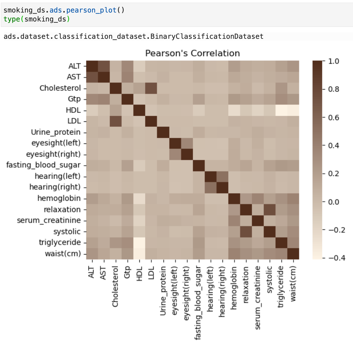
Correlation plots: Oracle ADS has 3 built in correlation methods for quick analysis and correlation plots. These correlation methods depend on the type of data that you're working with. For continuous numerical variables you would use Pearson correlation df.ads.pearson(); to compare categorical variables to continuous variables you would use the Correlation ratio df.ads.correlation_ratio(); and to measure the amount of association between two categorical variables you would use Cramer's V df.ads.cramersv().  Each of these have an associated plot function to visualise the correlations for example df.ads.pearson_plot() where “df” in these examples can be a pandas data frame or an ADS dataset.

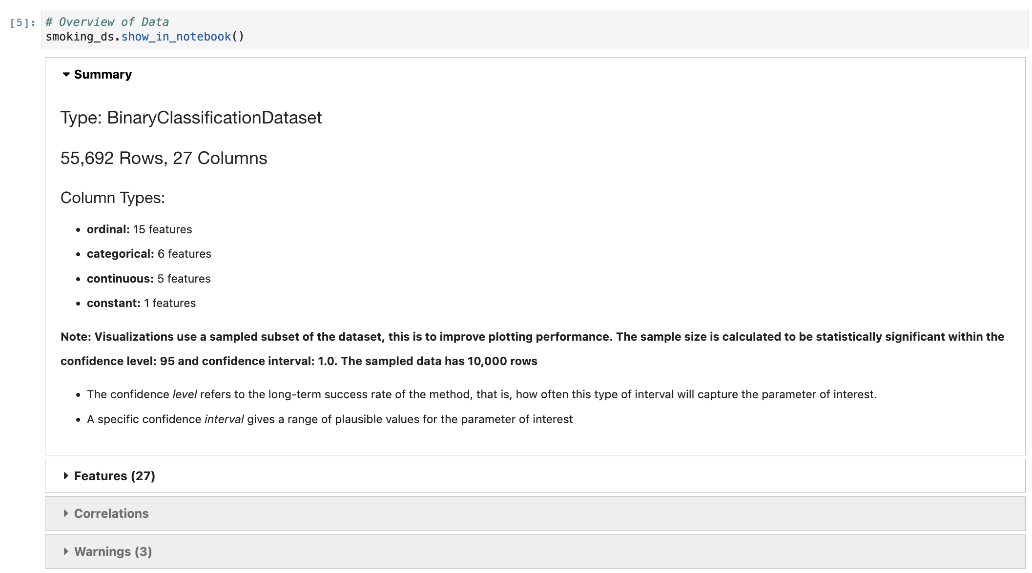
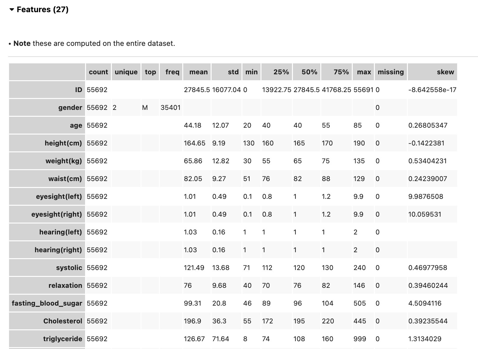
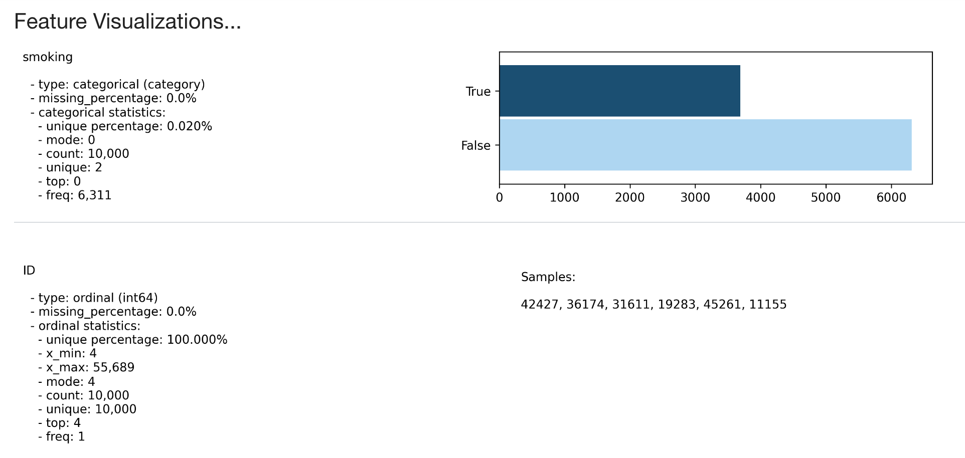
Show in notebook: The ADS show_in_notebook method creates a preview of all the basic information about the data set. It gives a great overview of what's in the data, number of rows and columns, data types/feature types of each column, visualisations of each column, correlations, and warnings about columns, for example columns that are mostly empty, or highly skewed columns. You can apply the ADS show_in_notebook method on an ads.dataset but not directly on a pandas data frame. More information about this can be found here: ADS Datasets, show_in_notebook.

Below is the output of the show_in_notebook function on the smoking dataset:

Cleaning and transforming data:

ADS has built-in functions to transform and manipulate data. The following work on ADS data sets, but any operation that can be performed on a pandas data frame can also be applied to an ADS data set.

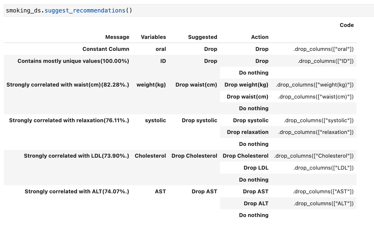
Suggest recommendations: The suggest_recommendations function highlights issues with the data and suggests changes to apply to the dataset that would make it more suitable for modelling. For example, dropping columns which are mostly empty, imputing missing values in a column with the most populous value, dropping a column if there is an additional highly correlated field. The output of this function is a table with the recommended changes, and  the code you could use to perform those steps.

Auto transform: If you wish to apply all the recommended changed from the suggest_recommendations function you can use auto_transform.  This function returns a transformed dataset, created from preforming all the recommendations at once.

transformed_smoking_ds = smoking_ds.auto_transform()

By default this will also handle imbalanced datasets by attempting to rebalance the data with up-sampling or down-sampling (although this can be turned off, and you can still use auto_transform to complete all other transformation steps).

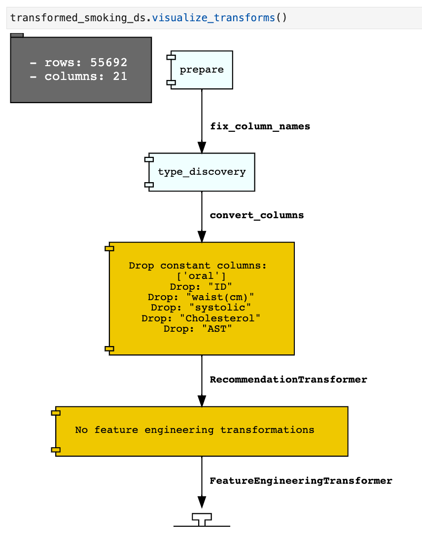
Visualize Transforms: If you have used auto_transform to preform the transformations you can use the visualize_transforms() function to view them. This function only works with the automated transformations and does not capture any custom transformations that you may have applied to the dataset.

transformed_smoking_ds.visualize_transforms()

Modelling

For the sake of brevity, in this blog I'm not going to be talking about Oracle's AutoML, which can be used within these notebooks via Oracle's AutoMLx package. I’m just going to run though creating two simple binary classifiers, and how they can be compared using ADS functions. As well as using additional ADS functions to deploy the model to the OCI Model catalogue, and load it back into a different notebook, we will also call a deployed model from and API.

In the examples below the following libraries are required :

# Required for creating and evaluating models 
from sklearn.datasets import make_classification
from sklearn.linear_model import LogisticRegression
from sklearn.ensemble import RandomForestClassifier
from sklearn.model_selection import train_test_split
from sklearn import metrics
from ads.common.model import ADSModel
from ads.evaluations.evaluator import ADSEvaluator
from ads.common.data import ADSData

Using the transformed smoking data set to create two binary classification models:

# Split the data into a training and test data set, here we are taking 15% of the data as the test data set and 85% as the training data set. 

train, test = transformed_smoking_ds.train_test_split(test_size=0.15)

# Splitting train and test X an y out for clarity
X_train = train.X
y_train = train.y
X_test= test.X
y_test = test.y

# Here we are using sklearn to train a Logistic Regression and a Random Forest Classifier Model.

# Logistic Regression Model
lr_clf = LogisticRegression(random_state=0, solver='lbfgs',
                    multi_class='multinomial').fit(X_train, y_train)

# Random Forest Model                   
rf_clf = RandomForestClassifier(n_estimators=100,
                                random_state=42).fit(X_train, y_train) 

Evaluating Models:

Models are only as useful as their quality of predictions. After training your model you will need to interpret its ability with a suitable evaluation metric. To do this in an unbiased way normally you would hold back a set of labelled data as an unseen test data set, this will enable you to assess the models performance by comparing the target and predicted values. You will then generate some metrics based on this to tell you how close the predicted values and target values are.

The evaluation metric which will be most suitable for your problem will depend on a range of things such as the type of model, binary classifier, multi class classifier, regression, as well as acceptable error margins, or if you wish to prioritise correctly predicting certain classes at the expense of others. Nevertheless, you will need a way to assess the performance of your created models and compare models with each other.

ADS Model evaluators: The ADSEvaluator and ADSModel class in the ADS package to generate a range of interpretable model metrics as standardised scores and charts. The metrics created will depend on the type of model used.

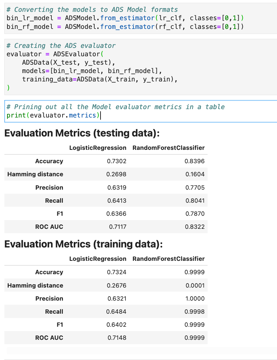
For example, here I am creating an ADS Evaluator. The ADS evaluator expects an ADS model format so first we convert our logistic regression and random forest model to ADS model formats.

# Converting the models to ADS Model formats
bin_lr_model = ADSModel.from_estimator(lr_clf, classes=[0,1])
bin_rf_model = ADSModel.from_estimator(rf_clf, classes=[0,1])

The function evaluator.metrics returns a table of metrics, you can also define and add your own metrics to this list using evaluator.add_metrics.

# Creating the ADS evaluator 
evaluator = ADSEvaluator(
    ADSData(X_test, y_test),
    models=[bin_lr_model, bin_rf_model],
    training_data=ADSData(X_train, y_train),
)

# Prining out the model evaluator metrics 
print(evaluator.metrics)

The list of returned metrics are dependent on the kind of model you have created, for example classification as opposed to regression. The evaluators for both of our binary classification models are shown below.

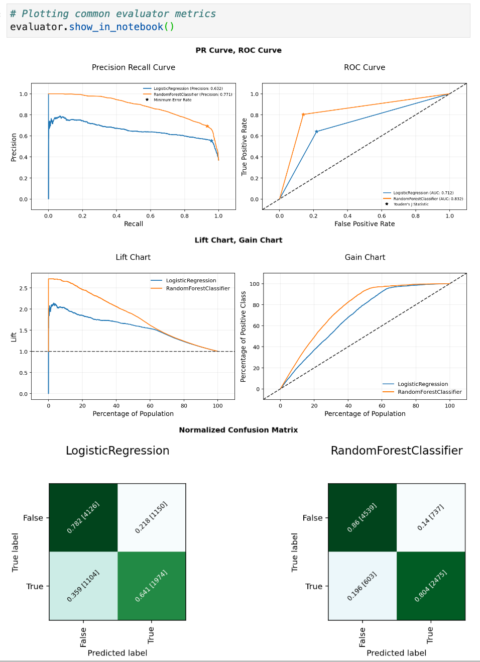
Evaluator with show in notebook: You can then use this evaluator with show in notebook to visualise a range of evaluation plots.

Here are some examples of charts created from the comparison of two binary classification models:

Saving and Deploying Models:

Once you have trained a suitable ML model for your use case, another common problem is how to version this model, and make it available for other people to utilise. Here we are going to use ADS to quickly prepare, save, and deploy a model. In the examples below the following libraries are required:

# Required for saving and deploying models 
from ads.model.framework.sklearn_model import SklearnModel
import tempfile
import json
from shutil import rmtree
from ads.model.model_metadata import UseCaseType

Preparing a Model:

The first step is to prepare the model, this involves creating a Model Artefact that contains the following items:

• A serialised model;
• runtime.yaml -  information about the model and required conda environment;
• score.py - used by the model deployment server to load in the model and create predictions;
• input_schema.json - Example input (optional);
• output_schema.json - Example output (optional);
• Any other artefacts required.

ADS can help us to auto generate all the mandatory files above to help save the models. Currently ADS supports the following frameworks:

• scikit-learn;
• XGBoost;
• LightGBM;
• PyTorch;
• SparkPipelineModel;
• TensorFlow.

There is also a GenericModel class that would help you to create the required files for any unsupported model framework that has a .predict()method.

Since the model we wish to save in this example is a scikit-learn model we can use the  SklearnModel class in ADS. The .prepare() function creates the model artefacts that are needed to deploy a model without you having to configure it or write code. However, it does allow you to customize the score.py file if needed.

The Model class takes two parameters - estimator object which is the model you wish to save and deploy and  a directory location to store autogenerated artefacts. The code below creates a temporary directory for the model artefacts, and sets the estimator to be the random forest model created above in this post.  To prepare the model we then provide information on the conda environment it should be run on, the conda environment it was trained in, the training data, and  the use_case_type: which will depend on the kind of model you have made and options available can be found on the Oracle ADS help page here.

In the example below since I am using a conda environment I created myself I’ve supplied the full path to the OCI bucket location.

artefact_dir = tempfile.mkdtemp()

sklearn_model = SklearnModel(estimator=rf_clf, artifact_dir=artefact_dir)
sklearn_model.prepare(
    inference_conda_env="oci://Bucket_Name@Namespace/conda_environments/cpu/RM_DS_ENV/1/rm_ds_envv1",
    training_conda_env="oci://Bucket_Name@Namespace/conda_environments/cpu/RM_DS_ENV/1/rm_ds_envv1",
    use_case_type=UseCaseType.BINARY_CLASSIFICATION,
    X_sample=X_train.head(5),
    y_sample=y_train.head(5),
    force_overwrite=True
)

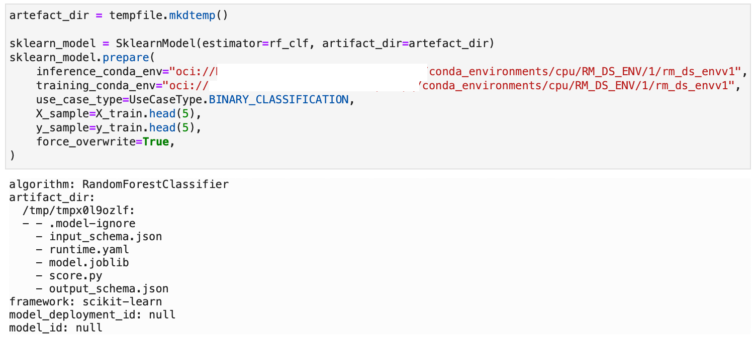
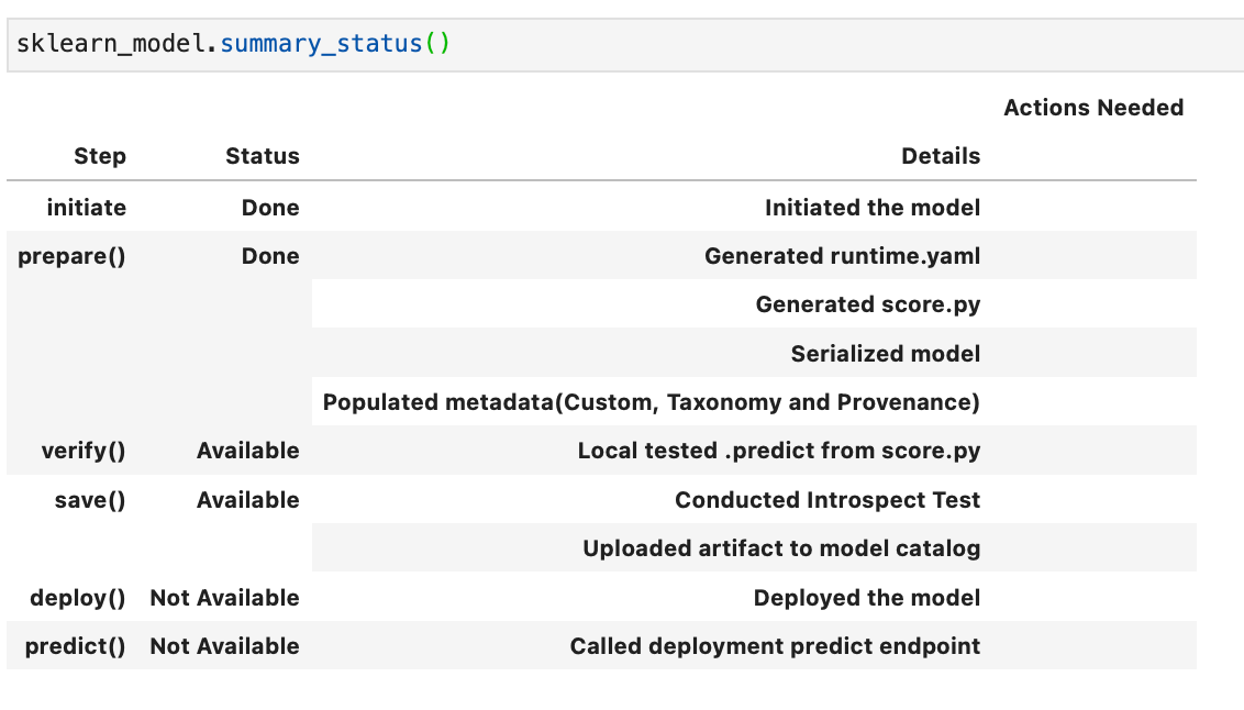
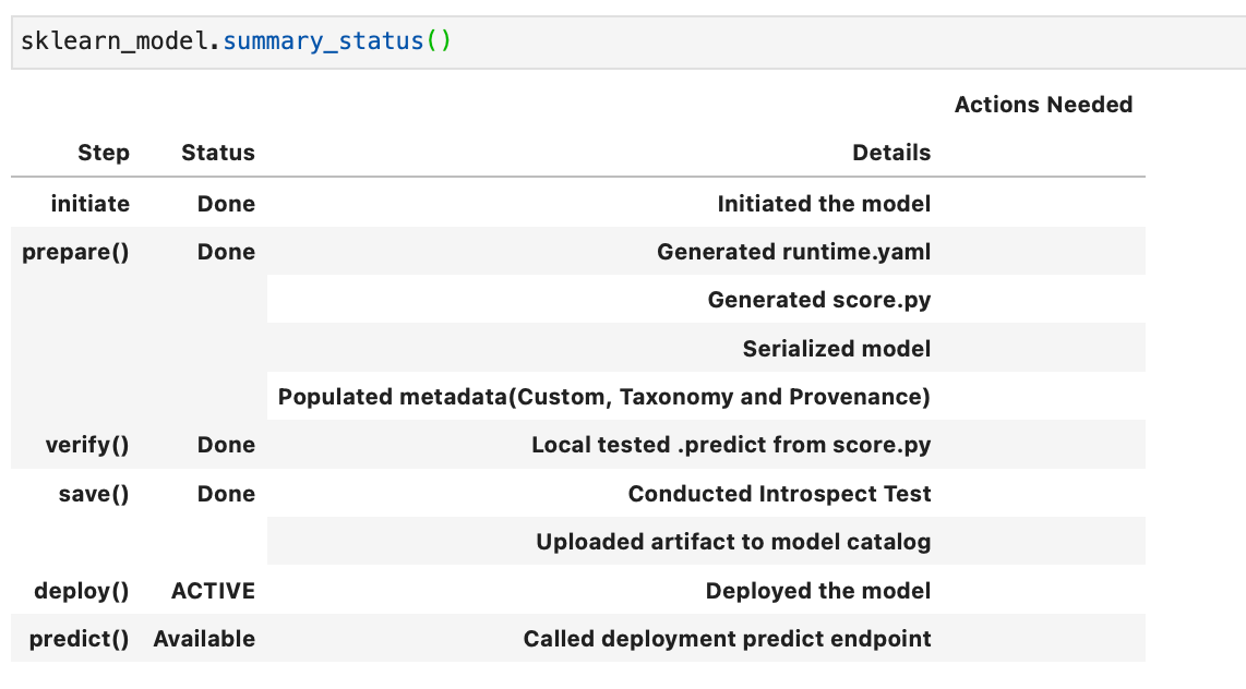
The above created the following files: runtime.yaml, score.py, and some json files with example inputs and outputs based around the sample training data sets supplied. If we use the  .summary_status() method we can see the steps required to deploy the model and which steps we have so far completed. Running this we can see that the next “Available” but not Done step is verify.

Verify a model: The .verify() method tests the score.py file with a sample of data. For example, below I am using the smoking test data set as a model input, and it returns a set of predictions.

sklearn_model.verify(X_test[:10])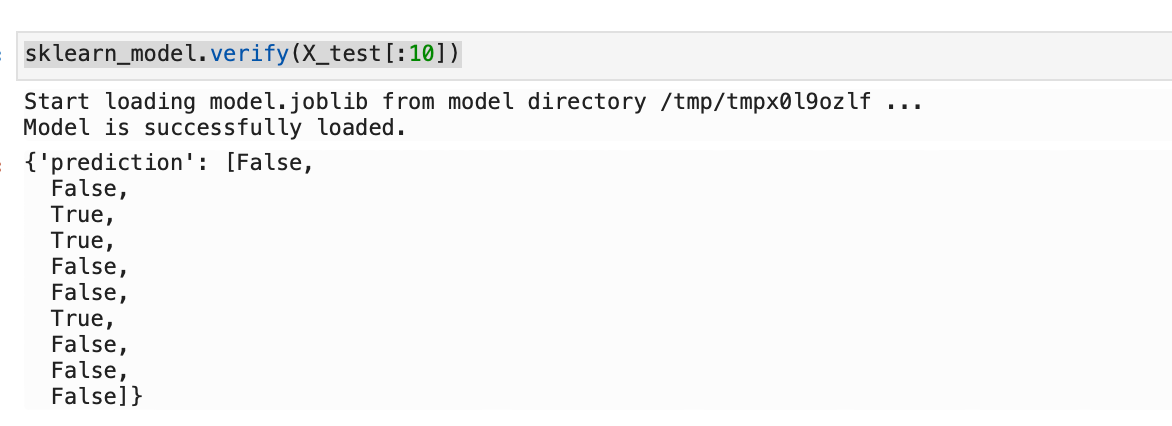

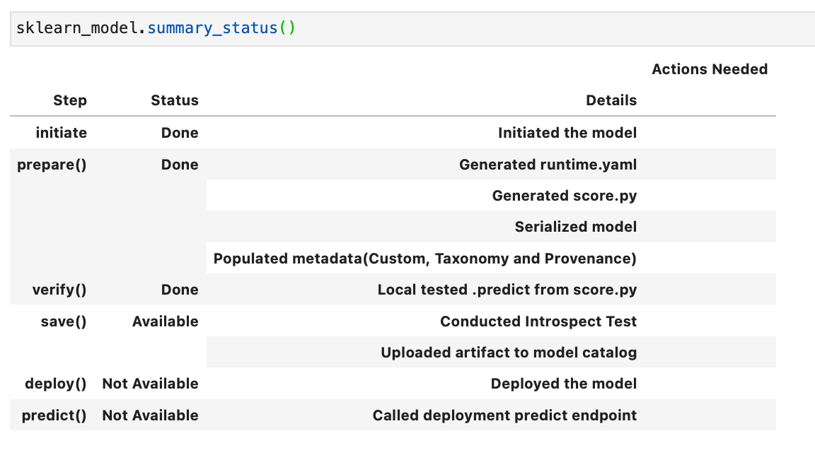
If we re-run  .summary_status() we can now see that the verify status is “Done”.

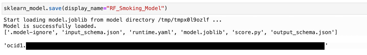
Saving a model to the model catalog: We can then use the .save() method to save the model to the OCI Model Catalog. This will fail if there is already a model with the supplied name saved to the catalog.

sklearn_model.save(display_name="RF_Smoking_Model")

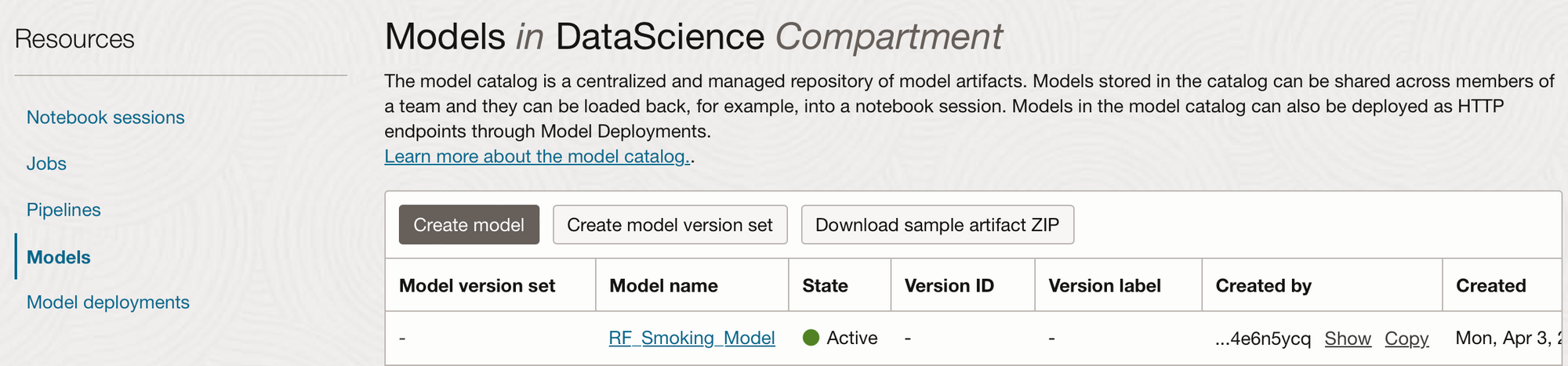
From the OCI Console we can now see our model in Analytics & AI -> Data Science -> Models.

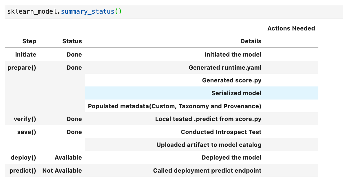
Model Deployments: Now that the model is saved to the catalogue, if we re-run .summary_status() we can now see that the save step is “Done” and the deploy step is “Available”. Deploying a model means that it is available from an HTTP endpoint that is hosted live on a compute node and is waiting to be called for predictions, it is active from the moment it is deployed until you deactivate it, and therefore you will be charged for the number of hours the model is deployed.

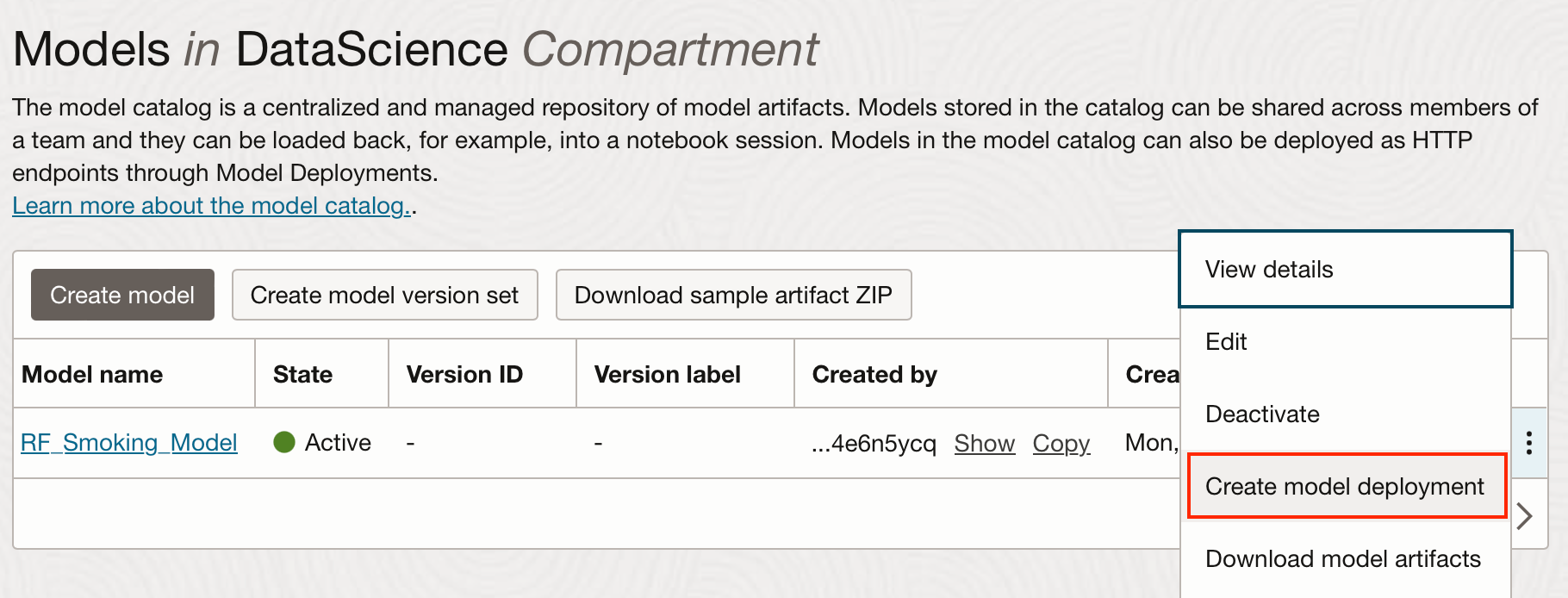
You can either deploy the model from the OCI console, by clicking on the 3 dots next to your saved model in the OCI model catalog, shown here:

Or from the notebook using the .deploy method:

deploy = sklearn_model.deploy(
    display_name="Random Forest Model For Smoking Classification",
    # instance_shape  = "VM.Standard2.1",
    # instance_count = 1,
    # project_id = "<PROJECT_OCID>",
    # compartment_id = "<COMPARTMENT_OCID",
    # access_log_group_id = "<ACCESS_LOG_GROUP_OCID>",
    # access_log_id = "<ACCESS_LOG_OCID>",
    # predict_log_group_id = "<PREDICT_LOG_GROUP_OCID>",
    # predict_log_id = "<PREDICT_LOG_OCID>"
)

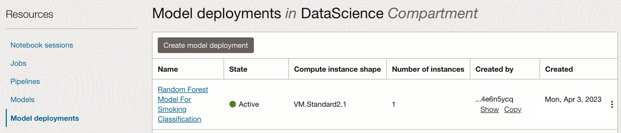
In the example above I have accepted all the default settings and only added a display name. You can however set the description, instance shape and count, set projects and compartments (defaults to the same as the notebook session), the maximum bandwidth, and logging groups. The .deploy() method returns a ModelDeployment object, and may take a few minutes to complete.  It can then be seen from the Model Deployments tab from within the OCI console.

Once the model is deployed the .predict method is available:

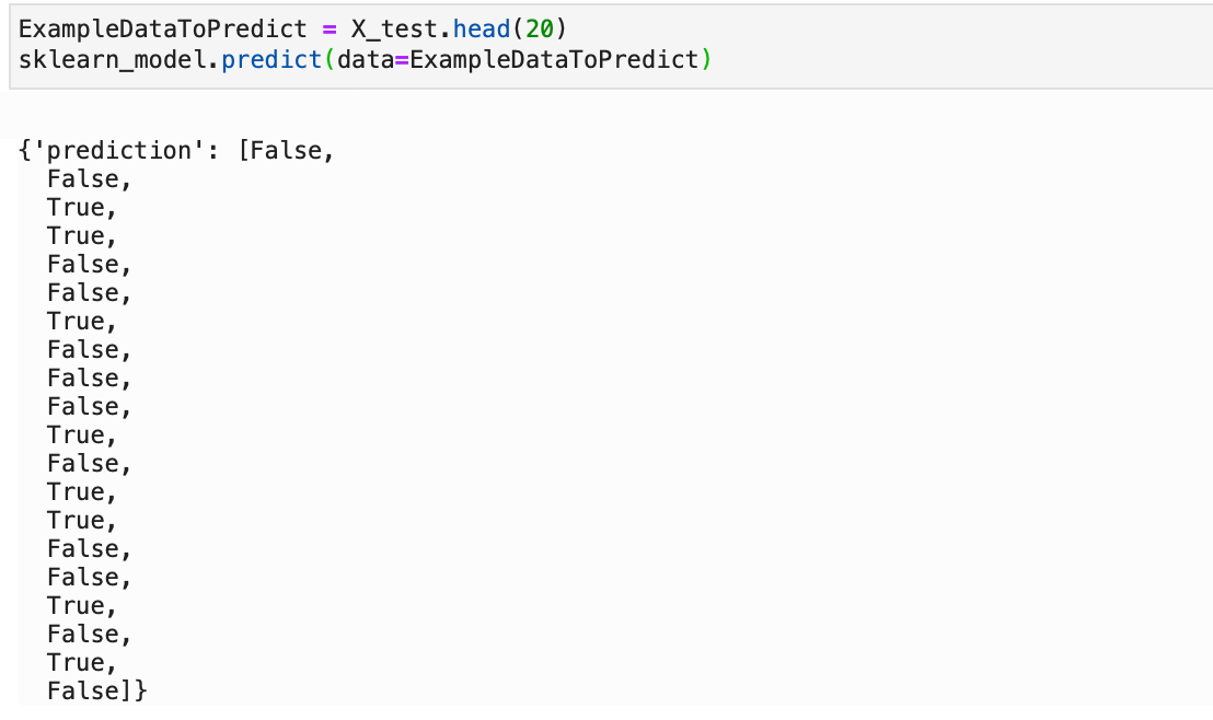
We can then use the .predict method on some data, here I'm using a subset of the test data.

ExampleDataToPredict = X_test.head(20)
sklearn_model.predict(data=ExampleDataToPredict)

Using Saved and Deployed Models:

Now that we have models that are saved and deployed in the OCI Model Catalog, how can we use them to create our predictions?

I’m going to show you several different ways to use the saved and deployed models. For example, if you wanted to load a saved, but not yet deployed model into any notebook session you can load it in with the following code:

# Change the OCID to the SAVED model OCID
saved_model = SklearnModel.from_model_catalog(
    "ocid1.datasciencemodel.oc1.xxx.xxxxx",
    model_file_name="model.joblib",
    artifact_dir="rf-download-test", # Directory for the model artefact files
)

# To create predictions from a model that isnt deployed, use verify. 
saved_model.verify(ExampleDataToPredict)["prediction"]

You could then create predictions using the .verify()  method, you can only use the .predict() method on deployed models. This might be worth considering if you want to create predictions in batch as opposed to adhoc, since you incur a cost for the hours your model is deployed.

If you or a different data scientist wanted to call the deployed model from within a notebook session they can load in the deployed model into their notebook session and then use the .predict() method as in the example below:

# Use the DEPLOPYMENT OCID
deployed_model = SklearnModel.from_model_deployment(
    "ocid1.datasciencemodel.oc1.xxx.xxxxx",
    model_file_name="model.joblib",
    artifact_dir="deployed-download-test", # Directory for the model artefact files
)

# To create predictions from deployed model
deployed_model.predict(ExampleDataToPredict)

Invoking the model from an HTTP endpoint

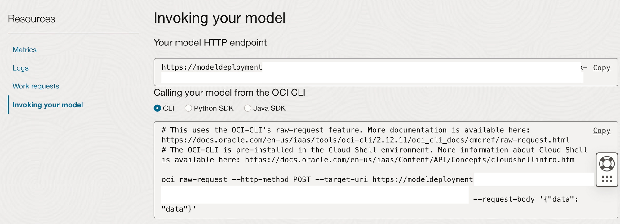
They can also call the model from the HTTP endpoint created when it was deployed. This endpoint could be used from anywhere that can invoke a REST API endpoint. There are some examples created when our model is deployed on how it can be called. In OCI if you navigate and click on your deployed model, you will see examples of how to invoke it from the CLI, Python, or Java.

For each of these options (except for the OCI Cloud Shell) you would first need to create an OCI credentials config file to allow you to authenticate to the tenancy hosting the deployment of the model. Information on how to create this config file can be found here.

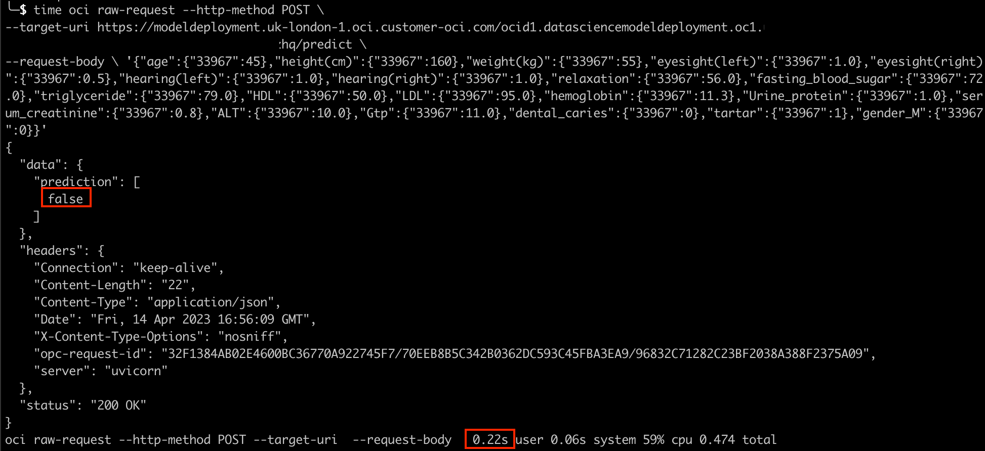
Once this config file has been created you can invoke this deployed model using the examples given on the OCI “Invoking your model” tab. Below I have already created an OCI config file on my Mac, I can therefore run the above code to create adhoc predictions by passing in a json payload in the command line.

oci raw-request --http-method POST \
--target-uri https://modeldeployment............./predict \
--request-body \
'{"age":{"33967":45},"height(cm)":{"33967":160},"weight(kg)":{"33967":55},
"eyesight(left)":{"33967":1.0},"eyesight(right)":{"33967":0.5},"hearing(left)":{"33967":1.0},
"hearing(right)":{"33967":1.0},"relaxation":{"33967":56.0},"fasting_blood_sugar":{"33967":72.0},
"triglyceride":{"33967":79.0},"HDL":{"33967":50.0},"LDL":{"33967":95.0},"hemoglobin":{"33967":11.3},
"Urine_protein":{"33967":1.0},"serum_creatinine":{"33967":0.8},"ALT":{"33967":10.0},"Gtp":{"33967":11.0},
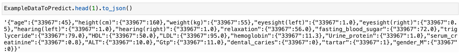
"dental_caries":{"33967":0},"tartar":{"33967":1},"gender_M":{"33967":0}}'

The json format supplied here was created from the training data set from within the OCI Notebook session we were using earlier.

ExampleDataToPredict.head(1).to_json()

Running this in the command line returned a prediction of “False” in 0.22 seconds.

Summary

In this post we've covered useful Oracle ADS functions for data exploration, as well as how we can create, save, deploy, and invoke models from within Oracle Data Science Notebook Sessions.

Coming up in Part 4:

Now we have created and deployed models we will quickly look at OCI Data Science Jobs and how these can be scheduled through OCI Data Integration Services.