Extended Visualisation of OBIEE Performance Data with Grafana

Recently I wrote about the new obi-metrics-agent tool and how it enables easy collection of DMS data from OBIEE into whisper, the time-series based database behind graphite. In this post I’m going to show two things that take this idea further:

1. How easy it is to add other data into Graphite
2. How to install and use Grafana, a most excellent replacement for the graphite front-end.

Collecting data in Graphite

One of the questions I have been asked about using Graphite for collecting and rendering OBIEE DMS metrics is a very valid one : given that OBIEE is a data visualisation tool, and that it usually sits alongside a database, where is the value in introducing another tool that apparently duplicates both data storage and visualisation.

My answer is that it is horses for courses. Graphite has a fairly narrow use-case but what it does it does superbly. It lets you throw any data values at it (as we’re about to see) over time, and rapidly graph these out alongside any other metric in the same time frame.

You could do this with OBIEE and a traditional RDBMS, but you’d need to design the database table, write a load script, handle duplicates, handle date-time arithmetic, build and RPD, build graphs – and even then, you wouldn’t have some of the advanced flexibility that I am going to demonstrate with Grafana below.

Storing nqquery.log response times in Graphite

As part of my Rittman Mead BI Forum presentation “No Silver Bullets - OBIEE Performance in the Real World”, I have been doing a lot of work examining some of the internal metrics that OBIEE exposes through DMS and how these correlate with the timings that are recorded in the BI Server log, nqquery.log, for example:

[2014-04-21T22:36:36.000+01:00] [OracleBIServerComponent] [TRACE:2] [USER-33] [] [ecid: 11d1def534ea1be0:6faf73dc:14586304e07:-8000-00000000000006ca,0:1:9:6:102] [tid: e4c53700] [requestid: c44b002c] [sessionid: c44b0000] [username: weblogic] -------------------- 
Logical Query Summary Stats: Elapsed time 5, Response time 2, Compilation time 0 (seconds) [[
]]

Now, flicking back and forth between the query log is tedious with a single-user system, and as soon as you have multiple reports running it is pretty much impossible to track the timings from the log with data points in DMS. The astute of you at this point will be wondering about Usage Tracking data, but for reasons that you can find out if you attend the Rittman Mead BI Forum I am deliberately using nqquery.log instead.

Getting data in to Graphite is ridiculously easy. Simply chuck a metric name, value, and timestamp, at the Graphite data collector Carbon, and that’s it. You can use whatever method you want for sending it, here I am just using the Linux commandline tool NetCat (nc):

echo "example.foo.bar 3 `date +%s`"|nc localhost 2003

This will log the value of 3 for a metric example.foo.bar for the current timestamp (date +%s). Timestamps are in Unix Time, which is the number of seconds since 1st Jan 1970. You can specify historical values for your metric too:

echo "foo.bar 3 1386806400"|nc localhost 2003

Looking in Graphite we can see the handle of test values I just sent through appear:

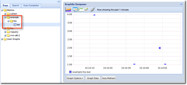
Tip: if you don’t see your data coming through, check out the logs in ~/graphite/storage/log/carbon-cache/carbon-cache-a/ (assuming you have Graphite installed in ~/graphite)

So, we know what data we want (nqquery.log timings), and how to get data into Graphite (send the data value to Carbon via nc). How do we bring the two together? We do this in the same way that many Linux things work, and that it using pipes to join different commands together, each doing one thing and one thing well. The above example demonstrates this - the output from echo is redirected to nc.

To extract the data I want from nqquery.log I am using grep to isolate the lines of data that I want, and then gawk to parse the relevant data value out of each line. The output from gawk is then piped to nc just like above. The resulting command looks pretty grim, but is mostly a result of the timestamp conversion into Unix time:

grep Elapsed nqquery.log |gawk '{sub(/\[/,"",$1);sub(/\]/,"",$1);sub(/\,/,"",$23);split($1,d,"-");split(d[3],x,"T");split(x[2],t,":");split(t[3],tt,".");e=mktime(d[1] " " d[2] " " x[1] " " t[1] " " t[2] " " tt[1]);print "nqquery.logical.elapsed",$23,e}'|nc localhost 2003

An example of the output of the above is:

nqquery.logical.response 29 1395766983
nqquery.logical.response 22 1395766983
nqquery.logical.response 22 1395766983
nqquery.logical.response 24 1395766984
nqquery.logical.response 86 1395767047
nqquery.logical.response 10 1395767233
nqquery.logical.response 9 1395767233

which we can then send straight to Carbon.

I’ve created additional versions for other available metrics, which in total gives us:

# This will parse nqquery.log and send the following metrics to Graphite/Carbon, running on localhost port 2003
#       nqquery.logical.compilation
#       nqquery.logical.elapsed
#       nqquery.logical.response
#       nqquery.logical.rows_returned_to_client
#       nqquery.physical.bytes
#       nqquery.physical.response
#       nqquery.physical.rows
# NB it parses the whole file each time and sends all values to carbon. 
# Carbon will ignore duplicates, but if you're working with high volumes 
# it would be prudent to ensure the nqquery.log file is rotated 
# appropriately.

grep Elapsed nqquery.log |gawk '{sub(/\[/,"",$1);sub(/\]/,"",$1);sub(/\,/,"",$23);split($1,d,"-");split(d[3],x,"T");split(x[2],t,":");split(t[3],tt,".");e=mktime(d[1] " " d[2] " " x[1] " " t[1] " " t[2] " " tt[1]);print "nqquery.logical.elapsed",$23,e}'|nc localhost 2003
grep Elapsed nqquery.log |gawk '{sub(/\[/,"",$1);sub(/\]/,"",$1);sub(/\,/,"",$26);split($1,d,"-");split(d[3],x,"T");split(x[2],t,":");split(t[3],tt,".");e=mktime(d[1] " " d[2] " " x[1] " " t[1] " " t[2] " " tt[1]);print "nqquery.logical.response",$26,e}'|nc localhost 2003
grep Elapsed nqquery.log |gawk '{sub(/\[/,"",$1);sub(/\]/,"",$1);split($1,d,"-");split(d[3],x,"T");split(x[2],t,":");split(t[3],tt,".");e=mktime(d[1] " " d[2] " " x[1] " " t[1] " " t[2] " " tt[1]);print "nqquery.logical.compilation",$29,e}'|nc localhost 2003
grep "Physical query response time" nqquery.log |gawk '{sub(/\[/,"",$1);sub(/\]/,"",$1);split($1,d,"-");split(d[3],x,"T");split(x[2],t,":");split(t[3],tt,".");e=mktime(d[1] " " d[2] " " x[1] " " t[1] " " t[2] " " tt[1]);print "nqquery.physical.response",$(NF-4),e}'|nc localhost 2003
grep "Rows returned to Client" nqquery.log |gawk '{sub(/\[/,"",$1);sub(/\]/,"",$1);split($1,d,"-");split(d[3],x,"T");split(x[2],t,":");split(t[3],tt,".");e=mktime(d[1] " " d[2] " " x[1] " " t[1] " " t[2] " " tt[1]);print "nqquery.logical.rows_returned_to_client",$(NF-1),e}'|nc localhost 2003
grep "retrieved from database" nqquery.log |gawk '{sub(/\[/,"",$1);sub(/\]/,"",$1);sub(/\,/,"",$(NF-9));split($1,d,"-");split(d[3],x,"T");split(x[2],t,":");split(t[3],tt,".");e=mktime(d[1] " " d[2] " " x[1] " " t[1] " " t[2] " " tt[1]);print "nqquery.physical.rows",$(NF-9),e}'|nc localhost 2003
grep "retrieved from database" nqquery.log |gawk '{sub(/\[/,"",$1);sub(/\]/,"",$1);split($1,d,"-");split(d[3],x,"T");split(x[2],t,":");split(t[3],tt,".");e=mktime(d[1] " " d[2] " " x[1] " " t[1] " " t[2] " " tt[1]);print "nqquery.physical.bytes",$(NF-7),e}'|nc localhost 2003

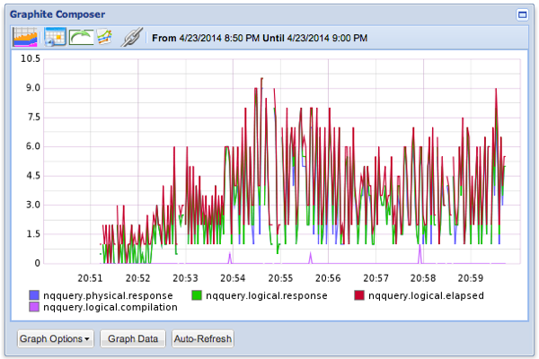
Now I run this script, it scrapes the data out of nqquery.log and sends it to Carbon, from where I can render it in Graphite:

Grafana

Grafana is an replacement for the default Graphite front-end, written by Torkel Ödegaard and available through the very active github repository.

It’s a great way to very rapidly develop and explore dashbaords of data sourced from Graphite. It’s easy to install too. Using SampleApp as an example, setup per the obi-metrics-agent example, do the following:

# Create a folder for Grafana
mkdir /home/oracle/grafana
cd /home/oracle/grafana
# Download the zip from http://grafana.org/download/
wget http://grafanarel.s3.amazonaws.com/grafana-1.5.3.zip
# Unzip it and rearrange the files
unzip grafana-1.5.3.zip
mv grafana-1.5.3/* .
# Create & update the config file
cp config.sample.js config.js
sed -i -e 's/8080/80/g' config.js
# Add grafana to apache config
sudo sed -i'.bak' -e '/Alias \/content/i Alias \/grafana \/home\/oracle\/grafana' /etc/httpd/conf.d/graphite-vhost.conf 
sudo service httpd restart 

# Download ElasticSearch from http://www.elasticsearch.org/overview/elkdownloads/
cd /home/oracle/grafana
wget https://download.elasticsearch.org/elasticsearch/elasticsearch/elasticsearch-1.1.1.zip
unzip elasticsearch-1.1.1.zip
# Run elasticsearch
nohup /home/oracle/grafana/elasticsearch-1.1.1/bin/elasticsearch &
# NB if you get an out of memory error, it could be a problem with the JDK available. Try installing java-1.6.0-openjdk.x86_64 and adding it to the path.

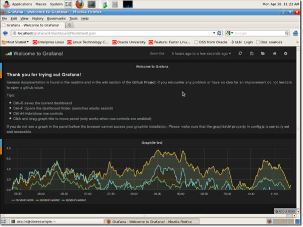
At this point you should be able to go to the URL on your sampleapp machine http://localhost/grafana/ and see the Grafana homepage.

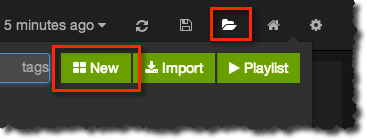
1. Click on the Open icon and then New to create a new dashboard

   

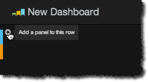
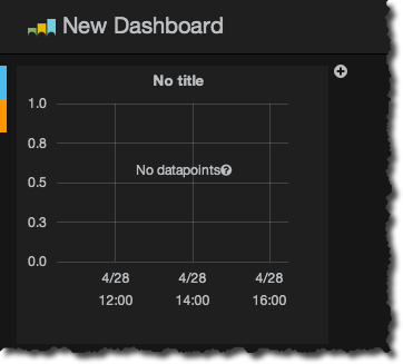
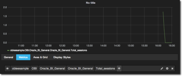
2. On the new dashboard, click Add a panel to this row, set the Panel Type to Graphite, click on Add Panel and then Close.
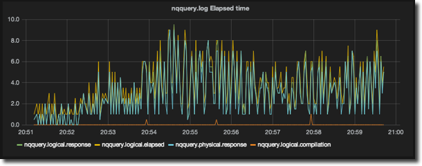
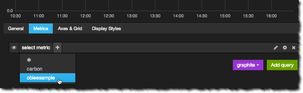
3. Click on the title of the new graph and select Edit from the menu that appears. In the edit screen click on Add query and from the select metric dropdown list define the metric that you want to display From here you can add additional metrics to the graph, or add graphite functions to the existing metric. I described the use of functions in my previous post about OBIEE and Graphite
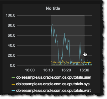
4. Click on Back to Dashboard at the top of the screen, to see your new graph in place. You can add rows to the dashboard, resize graphs, and add new ones. One of the really nice things you can do with Grafana is drag to zoom a graph, updating the time window shown for the whole page: 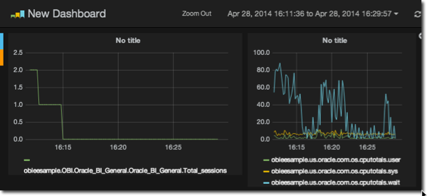You can set dashboards to autorefresh too, from the time menu at the top of the screen, from where you can also select pre-defined windows.
5. When it comes to interacting with the data being able to click on a legend entry to temporarily ‘mute’ that metric is really handy.

This really is just scratching the surface of what Grafana can do. You can see more at the website, and a smart YouTube video.

Summary

Here I’ve shown how we can easily put additional, arbitrary data into Graphite’s datastore, called Whisper. In this instance it was nqquery.log data that I wanted to correlate with OBIEE’s DMS data, but I’ve also used it very successfully in the past to overlay the number of executing JMeter load test users with other data in graphite.

I’ve also demonstrated Grafana, a tool I strongly recommend if you do any work with Graphite. As a front-end it is an excellent replacement for the default Graphite web front end, and it’s very easy to use too.