Spark Streaming and Kafka, Part 3 - Analysing Data in Scala and Spark

In my first two blog posts of the Spark Streaming and Kafka series - Part 1 - Creating a New Kafka Connector and Part 2 - Configuring a Kafka Connector - I showed how to create a new custom Kafka Connector and how to set it up on a Kafka server. Now it is time to deliver on the promise to analyse Kafka data with Spark Streaming.
When working with Apache Spark, you can choose between one of these programming languages: Scala, Java or Python. (There is also support for Spark querying in R.) Python is admittedly the most popular, largely thanks to Python being the most popular (and easiest to learn) programming language from the selection above. Python's PySpark library is catching up with the Spark features available in Scala, but the fact that Python relies on dynamic typing, poses challenges with Spark integration and in my opinion makes Spark a less natural fit with Python than with Scala.
Spark and Scala - the Basics
Spark was developed in Scala and its look and feel resembles its mother language quite closely. In fact, before diving into Spark Streaming, I am tempted to illustrate that for you with a small example (that also nicely recaptures the basics of Spark usage):
import org.apache.spark.rdd.RDD
import org.apache.spark.sql.SparkSession

object SparkTellDifference extends App {

    // set up Spark Context
    val sparkSession = SparkSession.builder.appName("Simple Application").config("spark.master", "local[*]").getOrCreate()
    val sparkContext = sparkSession.sparkContext
    sparkContext.setLogLevel("ERROR")

    // step 0: establish source data sets
    val stringsToAnalyse: List[String] = List("Can you tell the difference between Scala & Spark?", "You will have to look really closely!")
    val stringsToAnalyseRdd: RDD[String] = sparkContext.parallelize(stringsToAnalyse)

    // step 1: split sentences into words
    val wordsList: List[String]   = stringsToAnalyse    flatMap (_.split(" "))
    val wordsListRdd: RDD[String] = stringsToAnalyseRdd flatMap (_.split(" "))

    // step 2: convert words to lists of chars, create (key,value) pairs.
    val lettersList: List[(Char,Int)]   = wordsList    flatMap (_.toList) map ((_,1))
    val lettersListRdd: RDD[(Char,Int)] = wordsListRdd flatMap (_.toList) map ((_,1))

    // step 3: count letters
    val lettersCount: List[(Char, Int)] = lettersList groupBy(_._1) mapValues(_.size) toList
    val lettersCountRdd: RDD[(Char, Int)] = lettersListRdd reduceByKey(_ + _)

    // step 4: get Top 5 letters in our sentences.
    val lettersCountTop5: List[(Char, Int)] = lettersCount sortBy(- _._2) take(5)
    val lettersCountTop5FromRdd: List[(Char, Int)] = lettersCountRdd sortBy(_._2, ascending = false) take(5) toList

    // the results
    println(s"Top 5 letters by Scala native: ${lettersCountTop5}")
    println(s"Top 5 letters by Spark: ${lettersCountTop5FromRdd}")

    // we are done
    sparkSession.stop()
}
The code starts by setting up a Spark Session and Context. Please note that Spark is being used in local mode - I do not have Spark nodes installed in my working environment. With Spark Context set up, step 0 is to establish data sources. Note that the Spark RDD is based on the Scala native List[String] value, which we parallelize. Once parallelized, it becomes a Spark native.
Step 1 splits sentences into words - much like we have seen in the typical Spark word count examples. Step 2 splits those word strings into Char lists - instead of words, let us count letters and see which letters are used the most in the given sentences. Note that Steps 1 and 2 look exactly the same whilst the first one is Scala native whereas the second works with a Spark RDD value. Step 2 ends with us creating the familiar (key,value) pairs that are typically used in Spark RDDs.
Step 3 shows a difference between the two - Spark's reduceByKey has no native Scala analogue, but we can replicate its behaviour with the groupBy and mapValues functions.
In step 4 we sort the data sets descending and take top 5 results. Note minor differences in the sortBy functions.
As you can see, Spark looks very Scala-like and you may have to look closely and check data types to determine if you are dealing with Scala native or remote Spark data types.
The Spark values follow the typical cycle of applying several transformations that transform one RDD into another RDD and in the end the take(5) action is applied, which pulls the results from the Spark RDD into a local, native Scala value.
Introducing Spark Streaming
A good guide on Spark Streaming can be found here.
A quick overview of Spark Streaming with Kafka can be found here, though it alone will unlikely be sufficient to understand the Spark Streaming context - you will need to read the Spark Streaming guide as well.
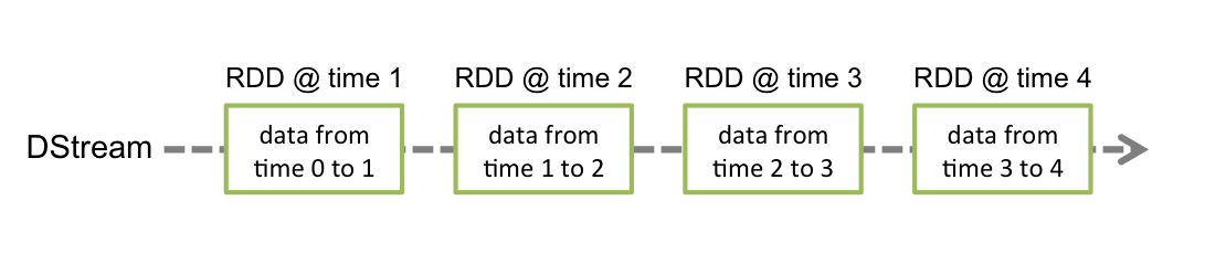
Working with Spark streams is mostly similar to working with regular RDDs. Just like the RDDs, on which you apply transformations to get other immutable RDDs and then apply actions to get the data locally, Spark Streams work similarly. In fact, the transformation part looks exactly the same - you apply a transformation on a Discretized Stream (DStream) to get another DStream. For example, you can have a val words: DStream[String] that represents a stream of words. You can define another DStream with those same words in upper case as
val wordsUpper: DStream[String] = words map (_.toUpperCase)Note that both these values represent streams - data sources where new data production might be ongoing. So if you have an incoming stream of words, you can define another data stream of the same words but in upper case. That includes the words not yet produced into the stream.
(If the values words were an RDD, the wordsUpper calculation would look almost the same: val wordsUpper: RDD[String] = words map (_.toUpperCase).) However, DStreams and RDDs differ when it comes to getting the data locally - for RDDs you call actions, for DStreams it is a bit more complicated. But... let us start from the beginning.
Setting up Spark Streaming
Much like a Spark Session and Context, Spark Streaming needs to be initialised.
We start by defining Spark Config - much like for SparkSession in the simple Spark example, we specify the application name and define the nodes we are going to use - in our case - local nodes on my developer workstation. (The asterisk means that Spark can utilise all my CPU threads.)
val sparkConfig =
  new SparkConf().setMaster("local[*]").setAppName("SparkKafkaStreamTest")
The next step is creating a Spark StreamingContext. We pass in the config defined above but also specify the Spark Streaming batch interval - 1 minute. This is the same as the production interval by our Connector set up in Kafka. But we could also define a 5 minute batch interval and get 5 records in every batch.
val sparkStreamingContext = new StreamingContext(sparkConfig, Minutes(1))Before we proceed, we would like to disable the annoying INFO messages that Spark likes to flood us with. Spark log level is set in Spark Context but we do not have SparkContext defined, do we? We only have StreamingContext. Well, actually, upon the creation of a StreamingContext, SparkContext is created as well. And we can access it via the StreamingContext value:
sparkStreamingContext.sparkContext.setLogLevel("ERROR")That is the Spark Streaming Context dealt with.
Setting up Access to Kafka
Setting up access to Kafka is equally straightforward. We start by configuring Kafka consumer:
val kafkaConfig = Map[String, Object](
    "client.dns.lookup" -> "resolve_canonical_bootstrap_servers_only",
    "bootstrap.servers" -> "192.168.1.13:9092",
    "key.deserializer" -> classOf[StringDeserializer],
    "value.deserializer" -> classOf[StringDeserializer],
    "group.id" -> "kafkaSparkTestGroup",
    "auto.offset.reset" -> "latest",
    "enable.auto.commit" -> (false: java.lang.Boolean)
)
The parameters given here in a Scala Map are Kafka Consumer configuration parameters as described in Kafka documentation. 192.168.1.13 is the IP of my Kafka Ubuntu VM.
Although I am referring to my Kafka server by IP address, I had to add an entry to the hosts file with my Kafka server name for my connection to work:
192.168.1.13 kafka-boxThe client.dns.lookup value did not have an impact on that.
The next step is specifying an array of Kafka topics - in our case that is only one topic - 'JanisTest':
val kafkaTopics = Array("JanisTest")Getting First Data From Kafka
We are ready to initialise our Kafka stream in Spark. We pass our StreamingContext value, topics list and Kafka Config value to the createDirectStream function. We also specify our LocationStrategy value - as described here. Consumer Strategies are described here.
val kafkaRawStream: InputDStream[ConsumerRecord[String, String]] =
        KafkaUtils.createDirectStream[String, String](
            sparkStreamingContext,
            LocationStrategies.PreferConsistent,
            ConsumerStrategies.Subscribe[String, String](kafkaTopics, kafkaConfig)
        )
What gets returned is a Spark Stream coming from Kafka. Please note that it returns Kafka Consumer record (key,value) pairs. The value part contains our weather data in JSON format. Before we proceed with any sort of data analysis, let us parse the JSON in a similar manner we did JSON parsing in the Part 1 of this blog post. I will not cover it here but I have created a Gist that you can have a look at.
The weatherParser function converts the JSON to a WeatherSchema case class instance - the returned value is of type DStream[WeatherSchema], where DStream is the Spark Streaming container:
val weatherStream: DStream[WeatherSchema] =
   kafkaRawStream map (streamRawRecord => weatherParser(streamRawRecord.value))
Now our data is available for nice and easy analysis.
Let us start with the simplest - check the number of records in our stream:
val recordsCount: DStream[Long] = weatherStream.count()The above statement deserves special attention. If you have worked with Spark RDDs, you will remember that the RDD count() function returns a Long value instead of an RDD, i.e. it is an action, not a transformation. As you can see above, count() on a DStream returns another DStream, instead of a native Scala long value. It makes sense because a stream is an on-going data producer. What the DStream count() gives us is not the total number of records ever produced by the stream - it is the number of records in the current 1 minute batch. Normally it should be 1 but it can also be empty. Should you take my word for it? Better check it yourself! But how? Certainly not by just printing the recordsCount value - all you will get is a reference to the Spark stream and not the stream content.
Displaying Stream Data
Displaying stream data looks rather odd. To display the recordsCount content, you need the following lines of code:
recordsCount.print()

...

sparkStreamingContext.start() // start the computation
sparkStreamingContext.awaitTermination() // await termination
The DStream value itself has a method print(), which is different from the Scala's print() or println() functions. However, for it to actually start printing stream content, you need to start() stream content computation, which will start ongoing stream processing until terminated. The awaitTermination() function waits for the process to be terminated - typically with a Ctrl+C. There are other methods of termination as well, not covered here. So, what you will get is recordsCount stream content printed every batch interval (1 minute in our example) until the program execution is terminated.
The output will look something like this, with a new record appearing every minute:
-------------------------------------------
Time: 1552067040000 ms
-------------------------------------------
1

-------------------------------------------
Time: 1552067100000 ms
-------------------------------------------
0

-------------------------------------------
Time: 1552067160000 ms
-------------------------------------------
1
Notice the '...' between the recordsCount.print() and the stream start(). You can have DStream transformations following the recordsCount.print() statement and other DStream print() calls before the stream is started. Then, instead of just the count, you will get other values printed for each 1 minute batch.
You can do more than just print the DStream content on the console, but we will come to that a bit later.
Analysing Stream Data
Above we have covered all the basics - we have initialised Spark Context and Kafka access, we have retrieved stream data and know how how to set up ongoing print of the results for our Stream batches. Before we proceed with our exploration, let us define a goal for our data analysis.
We are receiving a real-time stream of weather data. What we could analyse is the temperature change dynamics within the past 60 minutes. Note that we are receiving a new batch every minute so every minute our 60 minute window will move one step forward.
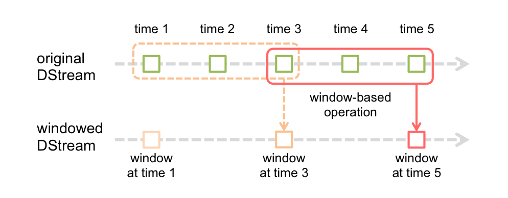
What we have got is our weatherStream DStream value. First let us define a Stream window of 60 minutes (check Spark documentation for explanation on how Stream Windows work.)
val weatherStream1Hour: DStream[WeatherSchema] = weatherStream.window(Minutes(60))The WeatherSchema case class contains many values. But all we need for our simple analysis is really just the timestamp and temperature. Let us extract just the data we need and put it in a traditional RDD (key,value) pair. And we print the result to verify it.
val weatherTemps1Hour: DStream[(String, Double)] =
   weatherStream1Hour map (weatherRecord =>
     (weatherRecord.dateTime, weatherRecord.mainTemperature)
   )

weatherTemps1Hour.print()
Please note that the above code should come before the sparkStreamingContext.start()call.
The result we are getting looks something like this:
-------------------------------------------
Time: 1552068480000 ms
-------------------------------------------
(08/03/2019 16:57:27,8.42)
(08/03/2019 16:57:27,8.42)
(08/03/2019 17:06:02,8.38)
(08/03/2019 17:06:02,8.38)
(08/03/2019 17:06:02,8.38)
(08/03/2019 17:06:02,8.38)
(08/03/2019 17:06:02,8.38)
(08/03/2019 17:06:02,8.38)
(08/03/2019 17:06:02,8.38)
(08/03/2019 17:06:02,8.38)
...
Notice the ellipse at the end. Not all records get displayed if there are more than 10.
Of course, we will get a new result printed every minute. However, the latest results will be at the bottom, which means they will be hidden if there are more than 10 of them. Also note that the weather data we are getting is actually not refreshed every minute but more like every 10 minutes. Our 1 minute batch frequency does not represent the actual frequency of weather data updates. But let us deal with those problems one at a time.
For me, vanity always comes first. Let me convert the (key,value) pair output to a nice looking narrative.
val weatherTemps1HourNarrative = weatherTemps1Hour map {
  case(dateTime, temperature) =>
    s"Weather temperature at ${dateTime} was ${temperature}"
}

weatherTemps1HourNarrative.print()
The result:
-------------------------------------------
Time: 1552068480000 ms
-------------------------------------------
Weather temperature at 08/03/2019 16:57:27 was 8.42
Weather temperature at 08/03/2019 16:57:27 was 8.42
Weather temperature at 08/03/2019 17:06:02 was 8.38
Weather temperature at 08/03/2019 17:06:02 was 8.38
Weather temperature at 08/03/2019 17:06:02 was 8.38
Weather temperature at 08/03/2019 17:06:02 was 8.38
Weather temperature at 08/03/2019 17:06:02 was 8.38
Weather temperature at 08/03/2019 17:06:02 was 8.38
Weather temperature at 08/03/2019 17:06:02 was 8.38
Weather temperature at 08/03/2019 17:06:02 was 8.38
...
We are still limited to the max 10 records the DStream print() function gives us. Also, unless we are debugging, we are almost certainly going to go further than just printing the records on console. For that we use the DStream foreachRDD function, which works similar to the map function, but does not return any data. Instead, whatever we do with the Stream data - print it to console, save it into a CSV file or database - that needs to take place within the foreachRDD function.
The foreachRDD Function
The foreachRDD function accepts a function as a parameter, which receives as its input a current RDD value representing the current content of the DStream and deals with that content in the function's body.
Ok, at long last we are getting some results back from our Spark stream that we can use, that we can analyse, that we know how to deal with! Let us get carried away!
weatherTemps1Hour foreachRDD { currentRdd =>
  println(s"RDD content:\n\t${currentRdd.collect().map{case(dateTime,temperature) => s"Weather temperature at ${dateTime} was ${temperature}"}.mkString("\n\t")}")

  val tempRdd: RDD[Double] = currentRdd.map(_._2)

  val minTemp = if(tempRdd.isEmpty()) None else Some(tempRdd.min())
  val maxTemp = if(tempRdd.isEmpty()) None else Some(tempRdd.max())

  println(s"Min temperature: ${if(minTemp.isDefined) minTemp.get.toString else "not defined"}")

  println(s"Max temperature: ${if(maxTemp.isDefined) maxTemp.get.toString else "not defined"}")

  println(s"Temperature difference: ${if(minTemp.isDefined && maxTemp.isDefined) (maxTemp.get - minTemp.get).toString}\n")
}
Here we are formatting the output and getting min and max temperatures within the 60 minute window as well as their difference. Let us look at the result:
RDD content:
	Weather temperature at 08/03/2019 16:57:27 was 8.42
	Weather temperature at 08/03/2019 16:57:27 was 8.42
	Weather temperature at 08/03/2019 17:06:02 was 8.38
	Weather temperature at 08/03/2019 17:06:02 was 8.38
	Weather temperature at 08/03/2019 17:06:02 was 8.38
	Weather temperature at 08/03/2019 17:06:02 was 8.38
	Weather temperature at 08/03/2019 17:06:02 was 8.38
	Weather temperature at 08/03/2019 17:06:02 was 8.38
	Weather temperature at 08/03/2019 17:06:02 was 8.38
	Weather temperature at 08/03/2019 17:06:02 was 8.38
	Weather temperature at 08/03/2019 17:06:02 was 8.38
	Weather temperature at 08/03/2019 17:06:02 was 8.38
	Weather temperature at 08/03/2019 17:06:02 was 8.38
	Weather temperature at 08/03/2019 17:17:32 was 8.28
	Weather temperature at 08/03/2019 17:17:32 was 8.28
	Weather temperature at 08/03/2019 17:17:32 was 8.28
	Weather temperature at 08/03/2019 17:17:32 was 8.28
	Weather temperature at 08/03/2019 17:17:32 was 8.28
	Weather temperature at 08/03/2019 17:17:32 was 8.28
	Weather temperature at 08/03/2019 17:17:32 was 8.28
	Weather temperature at 08/03/2019 17:17:32 was 8.28
	Weather temperature at 08/03/2019 17:17:32 was 8.28
	Weather temperature at 08/03/2019 17:17:32 was 8.28
	Weather temperature at 08/03/2019 17:30:52 was 8.28
	Weather temperature at 08/03/2019 17:30:52 was 8.28
	Weather temperature at 08/03/2019 17:30:52 was 8.28
	Weather temperature at 08/03/2019 17:30:52 was 8.28
	Weather temperature at 08/03/2019 17:30:52 was 8.28
	Weather temperature at 08/03/2019 17:30:52 was 8.28
	Weather temperature at 08/03/2019 17:30:52 was 8.28
	Weather temperature at 08/03/2019 17:30:52 was 8.28
	Weather temperature at 08/03/2019 17:30:52 was 8.28
	Weather temperature at 08/03/2019 17:30:52 was 8.28
	Weather temperature at 08/03/2019 17:30:52 was 8.28
	Weather temperature at 08/03/2019 17:37:51 was 8.19
	Weather temperature at 08/03/2019 17:37:51 was 8.19
	Weather temperature at 08/03/2019 17:37:51 was 8.19
	Weather temperature at 08/03/2019 17:37:51 was 8.19
	Weather temperature at 08/03/2019 17:37:51 was 8.19
	Weather temperature at 08/03/2019 17:37:51 was 8.19
	Weather temperature at 08/03/2019 17:37:51 was 8.19
	Weather temperature at 08/03/2019 17:37:51 was 8.19
	Weather temperature at 08/03/2019 17:37:51 was 8.19
	Weather temperature at 08/03/2019 17:37:51 was 8.19
	Weather temperature at 08/03/2019 17:37:51 was 8.19
	Weather temperature at 08/03/2019 17:51:10 was 8.1
	Weather temperature at 08/03/2019 17:51:10 was 8.1
	Weather temperature at 08/03/2019 17:51:10 was 8.1
	Weather temperature at 08/03/2019 17:51:10 was 8.1
	Weather temperature at 08/03/2019 17:51:10 was 8.1
	Weather temperature at 08/03/2019 17:51:10 was 8.1
	Weather temperature at 08/03/2019 17:51:10 was 8.1
	Weather temperature at 08/03/2019 17:51:10 was 8.1
	Weather temperature at 08/03/2019 17:51:10 was 8.1
	Weather temperature at 08/03/2019 17:51:10 was 8.1
	Weather temperature at 08/03/2019 18:01:10 was 7.99
	Weather temperature at 08/03/2019 18:01:10 was 7.99
	Weather temperature at 08/03/2019 18:01:10 was 7.99
Min temperature: 7.99
Max temperature: 8.42
Temperature difference: 0.4299999999999997
(Now there is no Time: 1552068480000 ms signature in our results printout because we are no longer using the DStream print() function).
However, I would like my analysis to be more detailed. It is time to involve Spark DataFrames.
Kafka Stream Data Analysis with Spark DataFrames
Just like in the previous statement, I need to extract Stream data with the currentRDD function. In fact, all the code that follows will be within the currentRDD function block:
weatherStream1Hour foreachRDD { currentRdd => {
... // the following code comes here
}
First, let us create a DataFrame from an RDD. Spark RDDs and DataFrames are two quite different representations of distributed data. And yet - look how simply the conversion works:
val spark =
   SparkSession.builder.config(currentRdd.sparkContext.getConf).getOrCreate()
import spark.implicits._

val simpleDF: DataFrame = currentRdd.toDF()
simpleDF.createOrReplaceTempView("simpleDF")
This trick works because our weatherStream1Hour DStream and consequently the currentRdd value that represents the Stream content, are based on the WeatherSchema case class. (data types - weatherStream1Hour: DStream[WeatherSchema] and currentRdd: RDD[WeatherSchema].) Therefore the currentRdd.toDF() implicit conversion works - Spark understands Scala case classes.
Once we have the DataFrame created, we can create a Temp view so we can query this DF with Spark SQL - that is what the createOrReplaceTempView function is for.
Let us start with the simplest queries - query the count(*) and the full content of the DataFrame:
val countDF: DataFrame = spark.sql("select count(*) as total from simpleDF")
countDF.show()

val selectAllDF = spark.sql("select * from simpleDF")
selectAllDF.show()
The result:
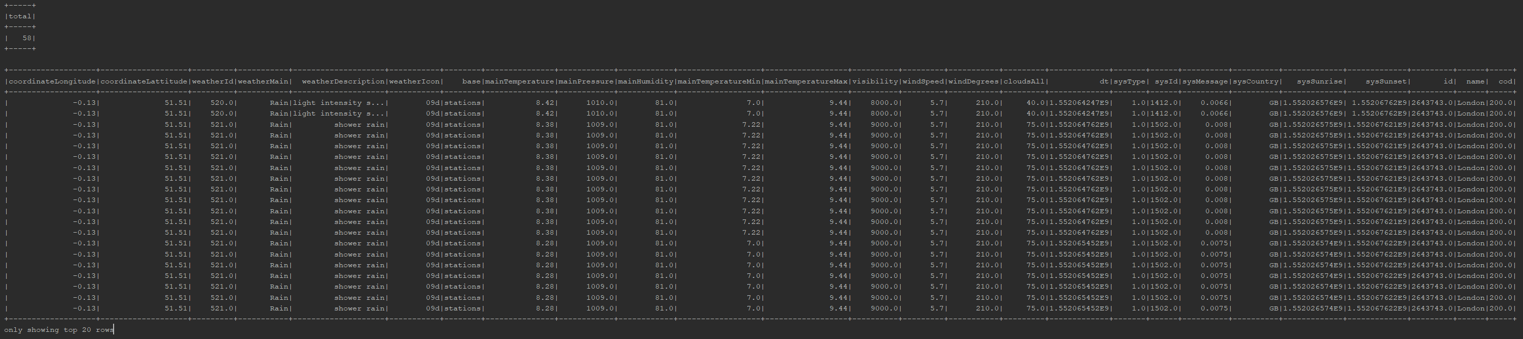
DataFrame's show() function by default only shows 20 rows, but we can always adjust that to show more or less. However, as we had established earlier in our analysis, the weather data actually does not get updated every minute - we are getting lots of duplicate records that we could get rid of. It is easy with SQL's distinct:
val distinctDF = spark.sql("select distinct * from simpleDF")
distinctDF.show()
The result - only 7 distinct weather measurements, confirming our suspicion that we are only getting a weather update approximately every 10 minutes:

Let us go back to our analysis - temperature change dynamics within the past 60 minutes. The temperature value in our DataFrame is named 'mainTemperature'. But where is the timestamp? We did have the dateTime value in our RDD. Why is it missing from the DataFrame? The answer is - because dateTime is actually a function. In RDD, when we referenced it, we did not care if it is a value or a function call. Now, when dealing with DataFrames, it becomes relevant.
As can be seen in the Gist, dateTime is a function, in fact it is a WeatherSchema case class method and is calculated from the dt value, which represents time in Unix format. The function that performs the actual conversion - dateTimeFromUnix - is defined in the WeatherParser object in the same Gist. If we want to get the save dateTime value in our DataFrame, we will have to register a Spark User Defined Function (UDF).
Creating a Spark User Defined Function (UDF)
Fortunately, creating UDFs is no rocket science - we do that with the Spark udf function. However, to use this function in a Spark SQL query, we need to register it first - associate a String function name with the function itself.
val dateTimeFromSeconds: Double => String = WeatherParser.dateTimeFromUnix(_)
val dateTimeFromSecondsUdf = udf(dateTimeFromSeconds)
spark.udf.register("dateTimeFromSecondsUdf", dateTimeFromSecondsUdf) // to register for SQL use
Now let us query the temperature and time:
val tempTimeDF = spark.sql(
"select distinct
dt timeKey,
dateTimeFromSecondsUdf(dt) temperatureTakenTime,
mainTemperature temperatureCelsius
from simpleDF order by timeKey"
)
tempTimeDF.show()
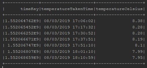
tempTimeDF.createOrReplaceTempView("tempTime")We show the results but also register the resulting DataFrame as a Temp View so we can from now on reference it in Spark SQL.
Note that we are converting the dt value to a String timestamp value but also keeping the original dt value - because dt is a number that can be sorted chronologically whereas the String timestamp cannot.
The result looks like this:
More Kafka Stream Data Analysis with Spark DataFrames
Now we have the times and the temperatures. But we want to see how temperatures changed between measurements. For example, between the two consecutive measurements at 17:06 and 17:17 the temperature (in London) dropped from 8.38 to 8.28 degrees Celsius. We want to have that value of minus 0.1 degrees in our result set.
If we were using Oracle database, the obvious choice would be the LAG analytic function. Do we have an analogue for that in Spark? Yes, we do! However, this time, instead of using Spark SQL, we will use the withColumn DataFrame function to define the LAG value:
val lagWindow = org.apache.spark.sql.expressions.Window.orderBy("timeKey")
val lagDF = tempTimeDF
  .withColumn("temperatureCelsiusPrev", lag("temperatureCelsius", 1, 0).over(lagWindow))
  .withColumn("rownum", monotonically_increasing_id())

lagDF.show()
lagDF.createOrReplaceTempView("tempTimeWithPrev")
The result:
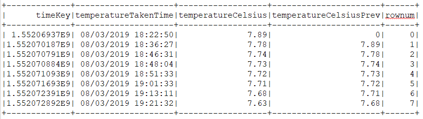
Here we are actually adding two values - lag and rownum, the latter being an analogue to the Oracle SQL ROW_NUMBER analytic function.
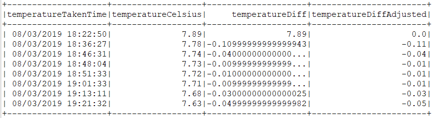
Note the inputs for the Spark lag function: The first is the source column name, the second is the lag offset and the third is default value - 0. The default value in our case will mean zero degrees Celsius, which will mess up our temperature delta for the first temperature measurement. Fortunately, Spark SQL also supports the CASE function so we can deal with this challenge with ease. In addition, let us round the result to get rid of the floating point artefacts.
val tempDifferenceDF = spark.sql(
	"select
		temperatureTakenTime,
		temperatureCelsius,
		temperatureCelsius - temperatureCelsiusPrev temperatureDiff,
		ROUND(CASE
			WHEN (rownum = 0)
			THEN 0
			ELSE temperatureCelsius - temperatureCelsiusPrev
		END, 2) AS temperatureDiffAdjusted
	from tempTimeWithPrev")

tempDifferenceDF.show()
And the result:
Conclusion
Kafka stream data analysis with Spark Streaming works and is easy to set up, easy to get it working. In this 3-part blog, by far the most challenging part was creating a custom Kafka connector. Once the Connector was created, setting it up and then getting the data source working in Spark was smooth sailing.
One thing to keep in mind when working with streams is - they are different from RDDs, which are static, immutable data sources. Not so with DStreams, which by their nature are changing, dynamic.
The challenging bit in the code is the
sparkStreamingContext.start() // start the computation
sparkStreamingContext.awaitTermination() // await termination
code block and its interaction with the foreachRDD function - to somebody not familiar with how Spark Streaming works, the code can be hard to understand.
The ease of creating a DataFrame from the original RDD was a pleasant surprise.
So, is using Spark and Kafka with Scala a good idea? Definitely yes. It works like a charm. However, in real life, additional considerations like the availability and cost of Python vs Scala developers as well as your existing code base will come into play. I hate real life.