Monitoring OBIEE with Elasticsearch, Logstash, and Kibana

Monitoring the health of an OBIEE system and diagnosing problems that may occur is a vital task for the system’s administrator and support staff. It’s one that at Rittman Mead we help customers with implementing themselves, and also provide as a managed service. In this article I am going to discuss the ELK stack, which fills a specific gap between the high-level monitoring and configuration functionality of Enterprise Manager 11g Fusion Middleware Control, and the Enterprise-grade monitoring, alerting and configuration management of Enterprise Manager 12c Cloud Control.
The ELK stack enables you to rapidly access both summary and detail information across the stack, supporting swift identification and diagnosis of any issues that may occur. The responsive interface lets you to drill into time periods or any ad-hoc field or filter as you wish, to analyse and diagnose problems. Data can be summarised and grouped arbitrarily, displaying relative error rates ensuring that genuine problems are not lost in the ‘noise’ of usual operation.


Out of the box, OBIEE ships with Enterprise Manager 11g Fusion Middleware Control (FMC), which as the name says is part of the Enterprise Manager line of tools from Oracle for managing systems. It is more of a configuration and deployment tool than it is really a monitoring and diagnostics one. The next step up is FMC’s (very) big brother, Enterprise Manager 12c Cloud Control (EM12c). This is very much its own product, requiring its own infrastructure and geared up to monitoring an organisation’s entire fleet of [Oracle] hardware and software. With this greatly enhanced functionally with EM12c also comes a license cost. The ELK stack conceptually fits perfectly alongside your existing EM FMC, providing a most excellent OBIEE monitoring dashboard and analysis tool, and allowing you to explore the kind of diagnostics and historical data that you could have access to in EM 12c.
In ELK we can see at a glance what kind of relative activity there has been on the system over the past few days:

There have been some errors, and the top three nQS and ORA error codes and messages are shown. This is an important differentiator to EM where you can search for errors, but cannot see straightaway if it is a one-off or multiple occurence. By grouping by error message it’s possible to quickly see what the biggest problem on a system may currently be:

At this point we might want to drill down into what was being run when the errors were being thrown. For example, from the error summary alone we can see the biggest problem was a locked database account - but which database was being queried? Lower down the dashboard page is a list of log details, and by clicking on the search icon against an error message we can filter the results shown:

We can use the search icon again to restrict results by ECID

And from there see all the related log entries, including which connection pool the request was against (and thus which database account is locked)

Another way of diagnosing a sudden rash of errors would be to instead drilldown on time alone to take a more holistic view at the logs (useful also given that ECIDs don’t always give the full picture). Using the system activity timeline along with the events log view it is a piece of cake to do this - simply click and drag a time window on the chart to instantly zoom into it.
Taking a step back up, we can see at a glance which areas of the OBIEE metadata model (RPD) are being used, as well as where we are pulling logs from – and all of these are clickable in order to filter the results further. So it’s easy to see, for a given subject area, what’s the current error rate? Or to quickly access all the log files for a specific set of components alone (for example, BI Server and OPMN). Any field that is displayed, whether in a chart or a detailed log view, can be clicked and used as the input for an ad-hoc filter.

It’s not just errors and logs we can monitor - the current and trending performance of the system (or a part of it; note the filtering by subject area and database described above) can be observed and of course, drilled into:

The ELK stack
The ELK stack is a suite of free software made up of three tools, the first letter of each giving it its name:
- ElasticSearch
- Logstash
- Kibana
At a very high level, we collect and enrich diagnostic data from log files using logstash, store it in ElasticSearch, and present and analyse it through Kibana.
- ElasticSearch is a document store, in which data with no predefined structure can be stored. Its origins and core strength are in full text search of any of the data held within it, and it is this that differentiates it from pure document stores such as MongoDB that Mark Rittman wrote about recently. Data is loaded and retrieved from ElasticSearch through messages sent over the HTTP protocol, and one of the applications that can send data this way and works extremely well is Logstash.
- Logstash is an innocuous looking tool that at first glance one could mistakenly write off as “just” a log parser. It does a lot more than that and a healthy ecosystem of input, filter, codec and output plugins means that it can interface between a great variety of applications, shifting data from one to another and optionally processing and enriching it along the way.
- The final piece of the stack is Kibana, a web application that enables one to build very flexible and interactive time-based dashboards, sourcing data from ElasticSearch. Interestingly, another of my favourite tools that I have written about before - and will write about again in this article - is Grafana which is forked from Kibana (and modified to source its data from time-series databases like graphite/carbon/whisper or InfluxDB) – thus if you’re at home with one you will be the other.

In this article I’m going to show how to set up your own ELK stack to monitor OBIEE, based on SampleApp v406.
Who is this for?
As you will see below, setting up and configuring the ELK stack does involve rolling up ones sleeves and diving right in. If you’re looking for an off-the-shelf monitoring solution then you should look elsewhere (such as EM12c). But if you want to have a crack at it I think you’ll be pleasantly surprised at what is possible once you get past the initially (bumpy) learning curve. The capabilities are great, and there’s an active support community as is the case with lots of open-source tools. With a bit of work it is possible to create a monitoring environment tailored pretty much entirely to your design.
Installing the stack
ELK runs on all common linux distributions (including Oracle Linux), as well as Mac OS. The only prerequisite is a JDK for ElasticSearch and Logstash, and web server for Kibana; here I am using Apache.
First up, let’s install JDK 1.7 (SampleApp has 1.6, which isn’t enough):
sudo yum install -y java-1.7.0-openjdk.x86_64
Apache is already installed on SampleApp, which we can verify thus:
[oracle@demo ~]$ sudo yum install -y httpd
Loaded plugins: refresh-packagekit
Setting up Install Process
Package httpd-2.2.15-29.0.1.el6_4.x86_64 already installed and latest version
Nothing to do
[oracle@demo ~]$ sudo service httpd status
httpd is stopped
It’s shutdown by default and that’s fine because we need to update the configuration on it anyway.
ElasticSearch
The easiest way to install ElasticSearch is using the yum repository:
sudo rpm --import http://packages.elasticsearch.org/GPG-KEY-elasticsearch

cat > /tmp/elasticsearch.repo<<EOF
[elasticsearch-1.3]
name=Elasticsearch repository for 1.3.x packages
baseurl=http://packages.elasticsearch.org/elasticsearch/1.3/centos
gpgcheck=1
gpgkey=http://packages.elasticsearch.org/GPG-KEY-elasticsearch
enabled=1
EOF

sudo mv /tmp/elasticsearch.repo /etc/yum.repos.d/
sudo yum install -y elasticsearch
I’d then set it to start at boot automagically:
sudo chkconfig elasticsearch on
and then start it up:
sudo service elasticsearch start
One final, optional, step in the installation is a plugin called kopf which gives a nice web dashboard for looking at the status of ElasticSearch:
export JAVA_HOME=/usr/lib/jvm/jre-1.7.0-openjdk.x86_64/
cd /usr/share/elasticsearch/bin
sudo ./plugin -install lmenezes/elasticsearch-kopf
logstash
There’s no repository for logstash, but it’s no biggie because there’s no install as such, just a download and unpack. Grab the download archive for logstash from the ELK download page, and then unpack it:
cd ~/Downloads
wget https://download.elasticsearch.org/logstash/logstash/logstash-1.4.2.tar.gz
# Need to use sudo because /opt is owned by root
sudo tar -xf logstash-1.4.2.tar.gz --directory /opt/
sudo mv /opt/logstash-1.4.2/ /opt/logstash/
sudo chown -R oracle. /opt/logstash/
Kibana
As with logstash, Kibana just needs downloading and unpacking. There’s also a wee bit of configuration to do, so that the web server (Apache, in our case) knows to talk to it, and so that Kibana knows how to find ElasticSearch.
cd ~/Downloads/
wget https://download.elasticsearch.org/kibana/kibana/kibana-3.1.0.tar.gz
sudo tar -xf kibana-3.1.0.tar.gz --directory /opt
sudo mv /opt/kibana-3.1.0/ /opt/kibana/
sudo chown -R oracle. /opt/kibana/
Now to configure Apache, telling it where to find Kibana. If you have existing sites configured, you’ll need to sort this bit out yourself, but on a vanilla SampleApp v406 you can use the following sed command to set up the needful:
sudo sed -i'.bak' -e 's/DocumentRoot.*$/DocumentRoot "\/opt\/kibana\/"/g' /etc/httpd/conf/httpd.conf
Lastly, Kibana needs to know where to find ElasticSearch, which is where it is going to pull its data from. An important point here is that the URL of ElasticSearch must be resolvable and accessing from the web browser you run Kibana on, so if you are using a DNS name it must resolve etc. You can update the configuratinon file config.js by hand (it’s the elasticsearch: definition that needs updating), or use this sed command:
sed -i'.bak' -e 's/^\s*elasticsearch:.*$/elasticsearch: "http:\/\/demo.us.oracle.com:9200",/g' /opt/kibana/config.js
Finally, [re]start Apache so that it uses the new configuration:
sudo service httpd restart
You should be able to now point your web browser at the server and see the default Kibana dashboard. So for sampleapp, if you’re running Firefox locally on it, the URL would simply be http://localhost/ (port 80, so no need to specify it in the URL). Note that if you’re doing anything funky with network, your local web browser needs to be able to hit both Apache (port 80 by default), and ElasticSearch (port 9200 by default).

Configuring ELK end-to-end
Now that we’ve got the software installed, let’s see how it hangs together and create our first end-to-end example. There’s a good logstash tutorial here that covers a lot of the functionality. Here, I’ll just look at some of the very basics, creating a very simple logstash configuration which will prompt for input (i.e. stdin) and send it straight to ElasticSearch. The kopf plugin that we installed above can show that the data made it to ElasticSeach, and finally we will create a very simple Kibana dashboard to demonstrate its use.
Logstash works by reading a configuration file and then running continually waiting for the configured input. As well as the input we configure an output, and optionally in between we can have a set of filters. For now we will keep it simple with just an input and output. Create the following file in /opt/logstash and call it logstash-basic.conf:
input {
        stdin {}
        }
output {
        elasticsearch {}
        }
It’s pretty obvious what it’s saying – for the input, use stdin, and send it as output to elasticsearch (which will default to the localhost).
Run this with logstash:
export JAVA_HOME=/usr/lib/jvm/jre-1.7.0-openjdk.x86_64/
cd /opt/logstash
bin/logstash -f logstash-basic.conf
After a few moments you should get a prompt. Enter some text, and nothing happens… apparently. What’s actually happened is that the text, plus some information such as the current timestamp, has been sent to ElasticSearch.

Let’s see where it went. In a web browser, got to http://localhost:9200/_plugin/kopf/. 9200 is the port on which ElasticSearch listens by default, and kopf is a plugin we can use to inspect ElasticSearch’s state and data. ElasticSeach has a concept of an index, in which documents, maybe of the same repeating structure but not necessarily, can be stored. Crudely put, this can be seen as roughly analogous to tables and rows of data respectively. When logstash sends data to ElasticSearch it creates one index per day, and in kopf now you should see an index with the current date, with a “document” for each line you entered after running logstash:

ElasticSearch can be queried using HTTP requests, and kopf gives a nice way to construct these and see the results which are in JSON format. Click on the rest (as in, REST API) menu option, leave the request as default http://localhost:9200/_search, and click send. You’ll see in the response pane a chunk of JSON in amongst which are the strings that you’ve entered to logstash:


Enter a few more lines into the logstash prompt, and then head over to http://localhost/ where you should find the default dashboard, and click on the Logstash Dashboard option:

It’s fairly bare, because there’s very little data. Notice how you have a histogram of event rates over the past day at the top, and then details of each event at the bottom. There are two things to explore here. First up, go and enter a bit more data into logstash, so that the create events have been spread out over time. Click the refresh icon on the Kibana dashboard, and then click-drag to select just the period on the chart that has data. This will zoom in on it and you’ll see in greater definition when the events were created. Go and click on one of the event messages in the lower pane and see how it expands, showing the value of each field – including message which is what logstash sent through from its input to output.

Now let’s get some proper data in, by pointing logstash at the BI Server log (nqsserver.log). Create a new configuration file, logstash-obi.conf, and build it up as follows. First we’ll use the file input to get data from …wait for it….a file! The syntax is fairly obvious:
input {
        file {
                path => "/app/oracle/biee/instances/instance1/diagnostics/logs/OracleBIServerComponent/coreapplication_obis1/nqserver.log"
                }
        }
Now we need to tell Logstash how to interpret the file. By default it’ll chuck every line of the log to ElasticSearch, with the current timestamp – rather than the timestamp of the actual event.

Now is time to introduce the wonderful world of the grok. A grok is one of the most important of the numerous filter plugins that are available in logstash. It defines expected patterns of content in the input, and maps it to fields in the output. So everything in a log message, such as the timestamp, user, ecid, and so on – all can be extracted from the input and stored as distinct items. They can also be used for further processing - such as amending the timestamp output from the logstash event to that of the log file line, rather than the system time at which it was processed.
So, let us see how to extract the timestamp from the log line. An important part of grok’ing is patterns. Grok statement are written as Regular expressions, or regex (obXKCD), so to avoid continual wheel-reinventing of regex statements for common objects (time, ip addresses, etc) logstash ships with a bunch of these predefined, and you can build your own too. Taking a line from nqsserver.log we can see the timestamp matches the ISO 8601 standard:

So our grok will use the pre-defined pattern TIMESTAMP_ISO8601, and then everything else (“GREEDYDATA”) after the timestamp, map to the log message field. The timestamp is in square brackets, which I’ve escaped with the backslash character. To indicate that it’s a grok pattern we want to match, it’s enclosed in %{ } markers.
\[%{TIMESTAMP_ISO8601:timestamp}\] %{GREEDYDATA:log_message}
This can be broken down as follows:
\[                                  The opening square bracket, escaped by \
%{TIMESTAMP_ISO8601:timestamp}      Capture an ISO 8601 timestamp, store it in a field called 'timestamp'
\]                                  The closing square bracket, escaped by \
%{GREEDYDATA:log_message}           Capture everything else ('GREEDYDATA' is also a grok pattern) and store it in the 'log_message' field
A grok operator in logstash is part of the filter processing, so we need a new stanza in the configuration file, after input and before output. Note that the grok operator is matching our pattern we built above against the message field, which is pre-populated by default by the input stream. You can grok against any field though.
input {
        file {
                path => "/app/oracle/biee/instances/instance1/diagnostics/logs/OracleBIServerComponent/coreapplication_obis1/nqserver.log"
                }
        }
filter {
        grok {
                match => ["message","\[%{TIMESTAMP_ISO8601:timestamp}\] %{GREEDYDATA:log_message}"]
            }
        }
output {
        elasticsearch {}
        }
Now we can see in the resulting capture we’ve extracted the timestamp to a field called “timestamp”, with the remainder of the field in “log_message”

But – the actual timestamp of the log entry that we have attached to the event stored in ElasticSearch, a special field called @timestamp is still reflecting the timestamp at which logstash read the logfile entry (30th September), rather than when the logfile entry was created (11th June). To fix this, we use a new filter option (grok being the first), the date filter:
date {
        match => ["timestamp", "yyyy-MM-dd'T'HH:mm:ss.SSSZZ"]
}
This matches the timestamp field that we captured with the grok, and converts it into the special @timestamp field of the event, using the mask specified. Now if we go back to kopf, the ElasticSearch admin tool, we can see that a new index has been created, with the date of log entry that we just parsed and correctly extracted the actual date from:

And over in Kibana if you set the timeframe long enough in the filter at the top you’ll be able to find the log entries showing up, now with the correct timestamp. Note that ElasticSearch accounts for the timezone of the message, storing it in UTC:

A large part of setting up your own ELK stack is this configuration of the filters in order to imbue and extract as much information from the log as you want. Grok filters are just the beginning – you can use conditional paragraphs to grok certain fields or logs for certain strings (think, error messages and ORA codes), you can mutate output to add in your own fields and tags based on what has been read. The point of doing this is that you enrich what is in the logs by giving the different pieces of data meaning that you can then drive the Kibana dashboard and filtering through.


Tips for using logstash
To think of the logstash .conf file as merely “configuration” in the same way a simple .ini is would be to underestimate it. In effect you are writing a bit of data transformation code, so brace yourself – but the silver lining is that whatever you want to do, you probably can. Logstash is a most flexible and powerful piece of software, and one in which the model of input, filter, codec and output work very well.
In the spirit of code development, here are some tips you may find useful:
- Grok patterns can inherit. Study the provided patterns (in the logstash patterns folder), and build your own. Look for commonality across files and look to reuse as much as possible. If you have multiple unrelated patterns for every type of log file in FMW then you’ve done it wrong.
- When you’re building grok statements and patterns, use the superb http://grokdebug.herokuapp.com. The advantage of this over a standard regex debugger is that it supports the grok syntax of capture groups and even custom patterns.
- For building up and testing regex from scratch, there are some useful sites: On the Mac there is a useful tool called Oyster which does the same as the above sites but doesn’t require an Internet connection.
- By default a failed grok will add the tag
_grokparsefailureto the event. If you have multiple grok clauses, give each its own uniquetag_on_failurevalue so that you can see from the output message which grok statement failed.grok { match => [ "message", "%{WLSLOG}" ] tag_on_failure => ["_grokparsefailure","grok03"] } - You can use
#as a comment character, so comment your code liberally, particularly whilst you’re finding your way with the configuration language so you can find your way back from the gingerbread house. - grok’ing takes resources, so target your grok statements by using conditionals. For example, to only parse nqquery logs for an expected string, you could write :
    if [path] =~ /nqquery/ {
    # Do your grok here
    }
NB the=~denotes a regex match, and the/delineate the regex string. - Use a conditional to split the output, writing and grok failures to stdout and/or a file, so that it is easier to see what’s failing and when. Note the use of the rubydebug codec here to prettify output sent to stdout.
output { if "_grokparsefailure" not in [tags] { elasticsearch { } } else { file { path => "unprocessed.out" } stdout { codec => rubydebug } } } - Use the multiline codec to work with log messages that span multiple lines, and watch out for newline characters – grok does not like them so use a mutate gsub to fix them out.
Building a Kibana dashboard
Now that we’ve got the data streaming through nicely from logstash into ElasticSearch, let us take a look at building dashboards against it in Kibana. Kibana is a web application that runs within an existing web server such as Apache, and it builds dashboards from data stored in ElasticSearch.
The building blocks of a Kibana dashboard are rows, which contain panels of a given pane width, up to twelve per row. On a panel goes one of the types of object, such as a graph. We’ll see now how to build up a dashboard and the interactions that we can use for displaying and analysing data.
When you first load Kibana you get a default dashboard that links to a few other start dashboards. Here we’re going to properly start from scratch so as to build up a picture of how a dashboard is created. Click on Blank Dashboard, and then in the top-right corner click on Configure Dashboard. Click on Index and from the Timestamping option select day. What this does is tell Kibana which ElasticSearch indices it is to pull data from, in this case using the standard Logstash index naming pattern - which we observed in kopf earlier - logstash-YYYY.MM.DD. Click Save, and then select Add a row. Give the row a title such as System Activity, click on Create Row and then Save. A new row appears on the dashboard.

Now we’ll add a graph to the row. Click on Add panel to empty row, and select Histogram as the Panel Type. Note that by default the width is 4 – change this to 12. You’ll note that there are plenty of options to explore, but to start with we’ll just keep it simple, so go ahead and click Save. By default the chart will show all data, so use the Time filter dropdown option at the top of the screen to select a recent time period. Assuming your data has loaded from logstash into ElasticSearch you should see a graph similar to this:

This is a graph of the number of events (log file entries) per time period. The graph will amend the resolution according to the zoom so that a reasonable resolution of data is shown, or you can force it through the Resolution option in the graph properties. In the legend of the chart you can see the resolution currently used.


Assuming you’ve selecting a broad time interval, such as the last week, you’ll presumably want to drill into the data shown. This is very intuitive in Kibana - simply click and drag horizontally over the time period you want to examine.

There are two important concepts for selecting and grouping data in Kibana, called filters and queries. A query groups data based on conditions, and we’ll explore those later. Filtering is a predicate applied to all data returned. Think of it just like a WHERE clause on a SQL query. You can see the current filter(s) applied at the top of the dashboard.

You may well want to hide these, and they can be collapsed - as can the query row and all of the dashboard rows - by clicking on the little triangle

From the Filter area you can also add, amend, disable and remove filters.
So far all we’ve got is a graph showing system activity over time, based on events recorded in a log file. But, we’ve no way of seeing what those logs are, and this is where the Table panel comes in. Add a new row, give it a title of Log messages and add the Table panel to it specifying the span as 12. You should now see a list of messages with timestamps corresponding to the time period shown in the graph. You can customise the Table panel, for example specifying which fields to show; by default it shows _source which is the raw row returned by ElasticSearch. More useful to us is the log_message field that we parsed out using the grok in logstash earlier. You can do this by selecting the relevant field from the Fields list on the left (which can be collapsed for convenience), or editing the Table panel and specifying it in the Columns area.


From the Table panel it is possible to select the data shown even more precisely by adding additional filters based on data in the table. Clicking on a particular row will expand it and show all of the associated fields, and each field has a set of Action options. You can filter only for that value, or specifically excluding it, and you can also add each field into the table shown (just like we did above for logmessage). So here I can opt to only display messages that I’ve tagged in logstash as coming from the BI Server component itself:


You’ll note in the second screenshow, once the filter has been applied, that the graph has changed and is showing less data. That is because a filter is global to a dashboard. But what if we want to show on the graph counts for all logs, but in the data table just those for BI Server? Here is where queries come into play. A query also looks like a predicate, but rather than restricting the data returned it just identifies a set of data within what is returned. To illustrate this I’m first going to remove all existing filters except the time period one:

And now in the Query area click on the + (to the right of the line). Now there are two queries, both with a wildcard as their value meaning they’ll each match everything. In the second query box I add the query Component: OracleBIServerComponent – note for this to work your logstash must be sending messages to ElasticSearch with the necessary Component field. Once updated, the second query’s impact can be seen in the graph, which is showing both the “all” query and the BI Server component tows. Use the View > option in the top left of the graph as a quick way of getting to the graph settings, including disabling cumulative/stack view:

Each panel in Kibana can be configured to show all or some of the query groups that have been defined. This is most useful for creating breakdowns of data, including those that are splitting it in different ways and you wouldn’t want all of the options displayed in entirety on all panels. You might want to group out the components, and the types of error, and then show a break down of system activity by one or the other – but not necessarily both. To configure which query a panel is to show use the Configure option in the top-right of a panel and go to the Queries tab. If it’s set to all then each and every query set will be shown individually on the panel.

If it’s selected then you can select one or more of the defined query sets to display

There are about a dozen types of panel in Kibana, and I’m not going to cover them all here. The other ones particularly of interest for building this kind of OBIEE monitoring dashboard include:
- Terms is basically a
SELECT FIELD, COUNT(*) ... GROUP BY FIELD. It shows the top x number of terms for a given field, and how frequently they occurred. Results can be as a pie or bar chart, or just a table: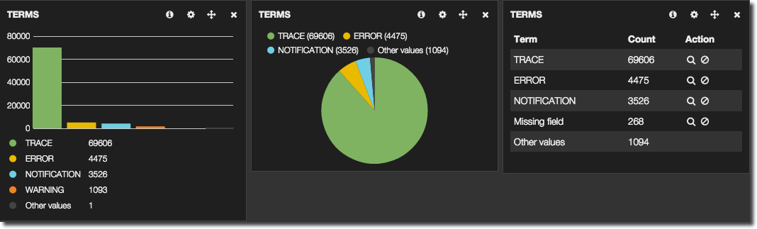 From a Terms panel you can add filters by clicking on a term. In the example above, clicking on the pie segment, or table row icon, for ERROR would add a filter to show just ERROR log entries
 - Trends shows the trend of event occurrences in a given time frame. Combined with an appropriate query you can show things like error rates

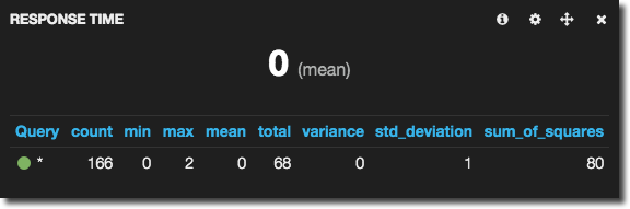
- Stats shows a set of statistics, so you can identify mean response times, maximum users logged on, and so on – assuming you have this data coming through from the logstash parsing.


Once you’ve built your dashboard save it (Kibana stores it in ElasticSearch). The dashboard is defined in json and you can opt to download this too.
The complete OBIEE monitoring view
Parsing logs is a great way to get out valuable information from the text stored and build visualisations and metrics on top of it. However, for pure metrics alone (such as machine CPU, OBIEE DMS metrics, and so on) a close-relation to Kibana, Grafana, is better suited to the task. Thus we have the text-based data going into ElasticSearch and reported through Kibana, and the pure metrics into a time-based store such as whisper (graphite’s database) and reported through Grafana. Because Grafana is a fork of Kibana, the look and feel is very similar.


Using obi-metrics-agent the DMS metrics from OBIEE can be collected and stored in whisper, and so also graphed out in Grafana alongside the system metrics. This gives us an overall architecture like this:

Obviously, it would be nice if we could integrate the fundamental time-based nature of both Kibana and Grafana together, so that drilling into a particular time period of interest maybe from an error rate point of view in the logs would also show the system and DMS metrics for the same period. There has been discussion about this (1, 2, 3) but I don’t get the impression that it will happen soon, if ever. One other item of interest here is Marvel, which is a commercial offering for monitoring ElasticSearch – through Kibana. It makes use of stock Kibana panel types, along with some new ones including the Nodes panel type, which suits the requirements we have of monitoring OBIEE/system metrics within a Kibana view, but unfortunately it looks like currently it is going to remain within Marvel only.

One other path to consider is trying to get the metrics currently sent to graphite/whisper instead into ElasticSearch so that Kibana can then report on them. The problem with this is twofold. Firstly, ElasticSearch is fundamentally a text-based store, whereas whisper fits much better for time/metric data (as would another DB such as influxDB). So trying to crow-bar the two together may not be the best solution, and instead better for it to be resolved at front end as discussed above. Secondly, Kibana’s graphing capabilities do not conceptually extend to multiple metrics in the same graph - only multiple queries - which means that graphing something that would be simple in Grafana (such as CPU wait/user/sys) would be overly complex in Kibana.
Architecting an ELK deployment
So far I’ve shown how to configure ELK on a single server, reading logs from that same server. But there are two extra things we should consider. First, Logstash in particular can be quite a ‘heavy’ process depending on how much work you’re doing with it. If you are processing all the logs that FMW writes, and have lots of grok filters (which isn’t a bad thing; it means you’re extracting lots of good information), then you will see logstash using a lot of CPU, lots IO, possibly to the detriment of other processes on the system - a tad ironic if the purpose of using logstash is to monitor for any system problems that occur. Secondly, ELK works very well with mutiple servers. You might have a scaled out OBIEE stack, or want to monitor multiple environments. Rather than replicating the ELK stack on each server instead it’s better for each server to push its log messages to a central ELK server for processing. And since the processing takes place on the ELK server and not the server being monitored we reduce the local resource footprint too.
To implement this kind of deployment, you need something like logstash-forwarder on the OBI server which is a light-touch program, sending the messages to logstash itself on the ELK server, over a custom protocol called lumberjack. Logstash then processes the messages as before, except it is reading the input from the logstash-forwarder rather than from file. An alternative approach to this is using redis as a message broker, with logstash running on both the source (sending output to redis) and ELK server (using redis as the input). This approach is documented very well here / here, and the former of using logstash-forwarder here. Logstash-forwarder worked very well for me in my tests, and seems to fit the purpose nicely.

Conclusion
Responsive monitoring tools are crucial for successful and timely support of an OBIEE system, and the ELK stack provides an excellent basis on which to build beyond the capabilities of Enterprise Manager Fusion Middleware Control. The learning curve is a bit steep at first, and you have to be comfortable with installing unpackaged tools, but the payoff makes it worth it! If you are interested in finding out about how Rittman Mead can help with your OBIEE implementation or other areas, please contact us.