Custom Machine Learning Models in Oracle DV

In a previous post, we’ve covered how to upload and execute custom Python scripts in Oracle Analytics Server (OAS), allowing greater flexibility in your data flows and more control over how your data are manipulated. However, executable scripts aren’t the only way to augment your OAS workflows using custom Python code; it’s also possible to upload custom machine learning models written using your machine learning library of choice. In this post, we’ll give a brief overview of how Python models can be trained and applied to data sources in OAS, as well as a glimpse of how Rittman Mead streamlines the process with custom script conversion tools.

Uploading XMLs

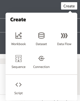
Custom models in OAS are uploaded by the same process as custom execution scripts, which was covered previously; Python code is embedded into an XML file, and uploaded to OAS by clicking Create on the Home screen and choosing the Script option.

This process is the generic method for uploading any custom file to OAS, and the XML fields detailed in the previous post are for files of the execute_script type. When these are added into a data flow, OAS will pass a dataset into the Python function, and expect an output dataframe with as many new or modified columns as the XML’s metadata instructs.

To upload a custom model instead, it is necessary to upload two separate XMLs; one to train the model, and another to apply it to data. This enables the user to re-use the training code and generate different instances of the model using different training data, data prepared with different cleaning pipelines, or different hyper parameters.

Custom Model Training Scripts

Custom model training scripts offer many of the same options and capabilities as custom execute scripts; they may specify an arbitrary number of named inputs to the script, import packages and modules from the Python environment, define functions externally to the main executable function, and run any arbitrary code in the body of the script. However, since these scripts are used to train models rather than manipulate data, there are two key differences between model training and custom execution scripts.

First, model training XMLs require the executable Python to be wrapped in a function named obi_create_model. Without this name, OAS will not recognise the script as the entry point to model training, and will therefore fail to execute. As with the obi_execute_script, obi_create_model takes three arguments:

• data: the input dataset as a pandas dataframe
• columnMetadata: metadata on the columns of data
• args: the optional input arguments as a dictionary

Second, we can only return one output: the model itself. This is intuitive enough, but does represent a constraint over and above the execute_script case, in which an arbitrary number of output columns could be specified. Additionally, the output model must be in the form of an obipy.obiml.Model.Model instance, which contains a pickled (serialised) copy of the custom model. This is how OAS stores the model for deployment.

The example script below shows how to train a simple random forest regressor on the iris dataset. Making use of custom input variables, we configure the script to train a model predicting a user selected sepal or petal dimension, and we can specify the number of estimators to include in the random forest.

First, we import the required packages and modules:

from sklearn.model_selection import train_test_split
from sklearn.ensemble import RandomForestRegressor
from sklearn.preprocessing import OneHotEncoder
import pandas as pd
import pickle
import base64

Next, we name our function obi_create_model and unpack the input arguments from args:

def obi_create_model(data, columnMetadata, args):

    target = str(args['Target'])
    n_est = int(args['n_estimators'])

The following code block generically trains a random forest regressor to predict our chosen target.

    X = data.loc[:, data.columns != target]
    y = data[target]
    cls = X['class']
    cls = cls.to_numpy()
    cls = cls.reshape(-1, 1)
    encoder = OneHotEncoder()
    cls_onehot = encoder.fit_transform(cls).toarray()
    df_onehot = pd.DataFrame(cls_onehot, columns=[f'class_{i}' for i in range(cls_onehot.shape[1])])
    X[list(df_onehot.columns)] = df_onehot
    X.drop(columns='class', inplace=True)

    X_train, X_test, y_train, y_test = train_test_split(X, y, test_size=0.2, random_state=42)
    rf_regressor = RandomForestRegressor(n_estimators=n_est, random_state=42)
    rf_regressor.fit(X_train, y_train)

Now we begin preparing the output, by defining which columns from data are to be included as necessary inputs for the model and storing them in the required_mappings dictionary.

    required_mappings = {}
    for col in data.columns:
        required_mappings[col] = 'true'

In order to store the trained model on OAS, we must pickle it. We can optionally include our input arguments in the pickle object so that the applying code knows which variable was the target and how many estimators were used.

    pickleobj={'RFRegression':rf_regressor, 'target': target, 'n_estimators':n_est}
    d = base64.b64encode(pickle.dumps(pickleobj)).decode('utf-8')

Finally, using the mappings and pickled model, we instantiate an obipy.obiml.Model.Model instance and return it:

    model = Model()
    model.set_data(__name__, 'pickle', d, target)
    model.set_required_attr(required_mappings)
    model.set_class_tag("Numeric")
    
    return model

Once this function and its required imports are embedded within an XML, with the script type, inputs and outputs defined appropriately, it is ready for upload. The example below shows our model training script embedded into an XML.

<?xml version='1.0' encoding='UTF-8'?>
<script>
  <scriptname>example_model.train</scriptname>
  <scriptlabel>example create rfr  (py)</scriptlabel>
  <target>python</target>
  <type>create_model</type>
  <scriptdescription><![CDATA[Trains a random forest regressor on the iris dataset to predict one of the petal or sepal dimensions based on  all other features]]></scriptdescription>
  <version>v1.1</version>
  <outputs/>
  <options>
    <option>
      <name>includeInputColumns</name>
      <displayName>Include Input Columns</displayName>
      <value>true</value>
      <required>false</required>
      <type>boolean</type>
      <hidden>true</hidden>
      <ui-config/>
    </option>
    <option>
      <name>Target</name>
      <displayName>Target</displayName>
      <required>true</required>
      <type>column</type>
      <value>sepalwidth</value>
      <description>Feature to predict</description>
      <hidden>false</hidden>
      <domain>
        <lov> value="sepalwidth" displayText="Sepal Width"</lov>
        <lov> value="petalwidth" displayText="Petal Width"</lov>
        <lov> value="sepallength" displayText="Sepal Length"</lov>
        <lov> value="petallength" displayText="Petal Length"</lov>
      </domain>
      <ui-config/>
    </option>
    <option>
      <name>n_estimators</name>
      <displayName>n_estimators</displayName>
      <required>true</required>
      <type>integer</type>
      <value>50</value>
      <description>Number of estimators in the random forest</description>
      <hidden>false</hidden>
      <domain> min="1" max="100"</domain>
      <ui-config/>
    </option>
  </options>
  <group>Machine Learning (Supervised)</group>
  <class>Custom</class>
  <algorithm>RandomForestRegressor</algorithm>
  <scriptcontent><![CDATA[""" Trains a random forest regressor on the iris dataset
to predict one of the petal or sepal dimensions based on 
all other features """
from sklearn.model_selection import train_test_split
from sklearn.ensemble import RandomForestRegressor
from sklearn.preprocessing import OneHotEncoder
import pandas as pd
import pickle
import base64

def obi_create_model(data, columnMetadata, args):

    target = str(args['Target'])
    n_est = int(args['n_estimators'])

    X = data.loc[:, data.columns != target]
    y = data[target]
    cls = X['class']
    cls = cls.to_numpy()
    cls = cls.reshape(-1, 1)
    encoder = OneHotEncoder()
    cls_onehot = encoder.fit_transform(cls).toarray()
    df_onehot = pd.DataFrame(cls_onehot, columns=[f'class_{i}' for i in range(cls_onehot.shape[1])])
    X[list(df_onehot.columns)] = df_onehot
    X.drop(columns='class', inplace=True)

    X_train, X_test, y_train, y_test = train_test_split(X, y, test_size=0.2, random_state=42)
    rf_regressor = RandomForestRegressor(n_estimators=n_est, random_state=42)
    rf_regressor.fit(X_train, y_train)

    required_mappings = {}
    for col in data.columns:
        required_mappings[col] = 'true'

    pickleobj={'RFRegression':rf_regressor, 'target': target, 'n_estimators':n_est}
    d = base64.b64encode(pickle.dumps(pickleobj)).decode('utf-8')

    model = Model()
    model.set_data(__name__, 'pickle', d, target)
    model.set_required_attr(required_mappings)
    model.set_class_tag("Numeric")

    return model]]></scriptcontent>
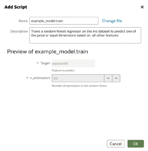
</script>

Using the Create menu we select the Script option and choose our training script. If the scriptdescription field is populated, this description will automatically be filled in the Add Script dialogue. We are also able to see the input arguments to our script and their default values.

Custom Model Apply Scripts

Next, we must produce a partner script to tell OAS how to generate and format a set of predictions using this model. Apply scripts must include a function named obi_apply_model, which takes the same three arguments as obi_execute_script and obi_create_model plus the additional model argument, the obipy.obiml.Model.Model instance created in obi_create_model.

Much like obi_execute_script,  obi_apply_model returns a dataframe, which may optionally have the input dataframe included. Typically, as a minimum, one of the returned columns will be the predicted values.

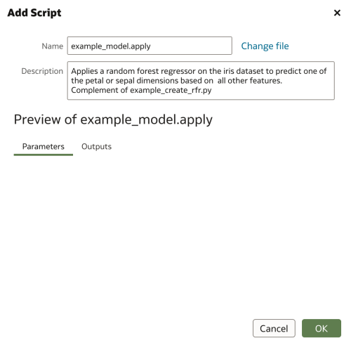
Finally, the create and apply scripts must have an identical base name, plus a ‘create’ or ‘apply’ label, such that OAS can associate them with one another. Our example XML files will be saved as example_model.create.xml and example_model.apply.xml.

Given the need to pre-process training and test data identically, the user may wish to isolate the data preparation steps away from the training and apply scripts, and instead include them as separate steps in their data flow, for example by utilising custom execute_scripts. This approach has the additional benefits of reducing duplicated code, and keeping the model training/applying scripts more focused and readable. For the sake of simplicity in this example, we instead replicate the data preparation steps in our apply script.

The example below shows how to apply our random forest regressor. Note that we are using the same set of data for both training and testing in this example. Obviously, this would not be the case in real applications.

As before, we start by importing the necessary packages and modules.

from sklearn.ensemble import RandomForestRegressor
from sklearn.preprocessing import OneHotEncoder
import pandas as pd

import pickle
import base64
from copy import deepcopy

We name our function as required and unpack our variables from their various containers. Our pickled model is extracted from model, unpickled, and then extracted into its own variable. We then extract our inputs from args and also unpack the inputs to obi_create_model by unpickling them from our model object. In this way, we are able to pass inputs directly from one script to another rather than replicating them.

def obi_apply_model(data, model, columnMetadata, args):

    pickleobj = pickle.loads(base64.b64decode(bytes(model.data, 'utf-8')))
    rfr_model = pickleobj['RFRegression']

    n_estimators = pickleobj['n_estimators']
    target = pickleobj['target']
    includeInput = args['includeInputColumns']

We make a copy of our input data and then verify that all required columns have been included.

    input_data = deepcopy(data)
    df = data

    required_mappings = model.required_attributes
    required_attributes = required_mappings.keys()

    apply_columns = df.columns
    if set(required_attributes) > set(apply_columns):
        raise ValueError('Required columns do not exist or have too many missing values.')

Here we repeat our data cleaning and preparation steps, ensuring that our test data are formatted exactly as our training data were. Once the data are prepared, we call the .predict() method and generate our predictions.

    X = data.loc[:, data.columns != target]
    cls = X['class']
    cls = cls.to_numpy()
    cls = cls.reshape(-1, 1)
    encoder = OneHotEncoder()
    cls_onehot = encoder.fit_transform(cls).toarray()
    df_onehot = pd.DataFrame(cls_onehot, columns=[f'class_{i}' for i in range(cls_onehot.shape[1])])
    X[list(df_onehot.columns)] = df_onehot
    X.drop(columns='class', inplace=True)

    preds = rfr_model.predict(X)
    pred_df = pd.DataFrame(preds.reshape(-1, 1), columns=['PredictedValue'])

Finally, we format our output dataframe to include or not include the input data, and then return our output.

    if includeInput.upper() == 'TRUE':
        output = pd.concat([pred_df, input_data], axis=1)
    else:
        output = pred_df

    return output

Again, all that remains is to embed the script in an XML, name it as required, and upload to OAS.

Training and Applying a Custom Model

With both scripts uploaded, we can now train our model and apply it to a test dataset.

We start by creating a new data flow. From the Home Screen, we click Create and then choose Data Flow.

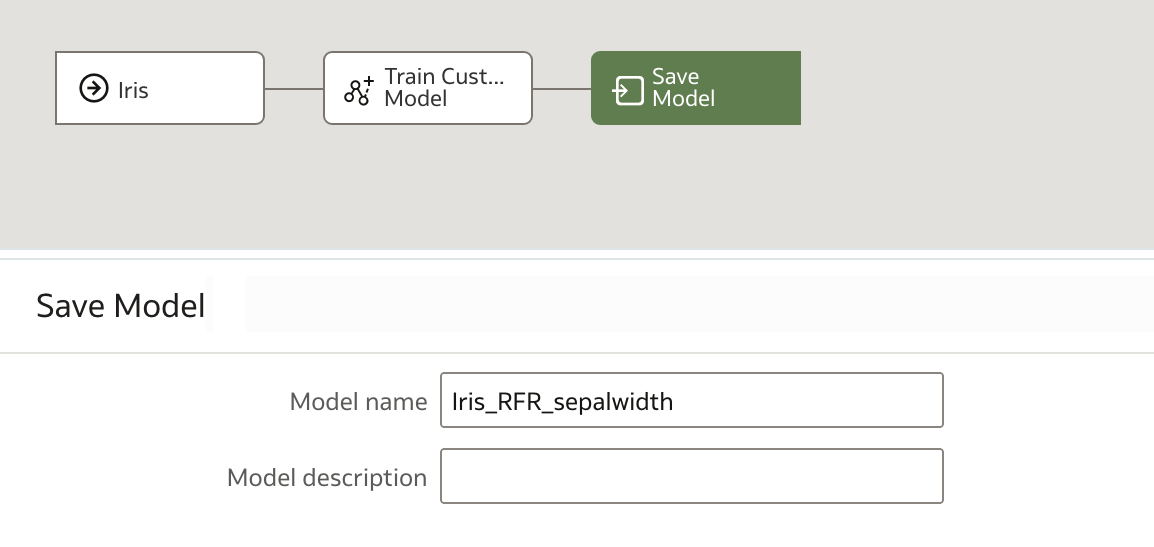
In our new data flow, we choose our training dataset, in this case, the iris dataset, and then choose Train Custom Model. From the dropdown box, we select our training script and then click OK.

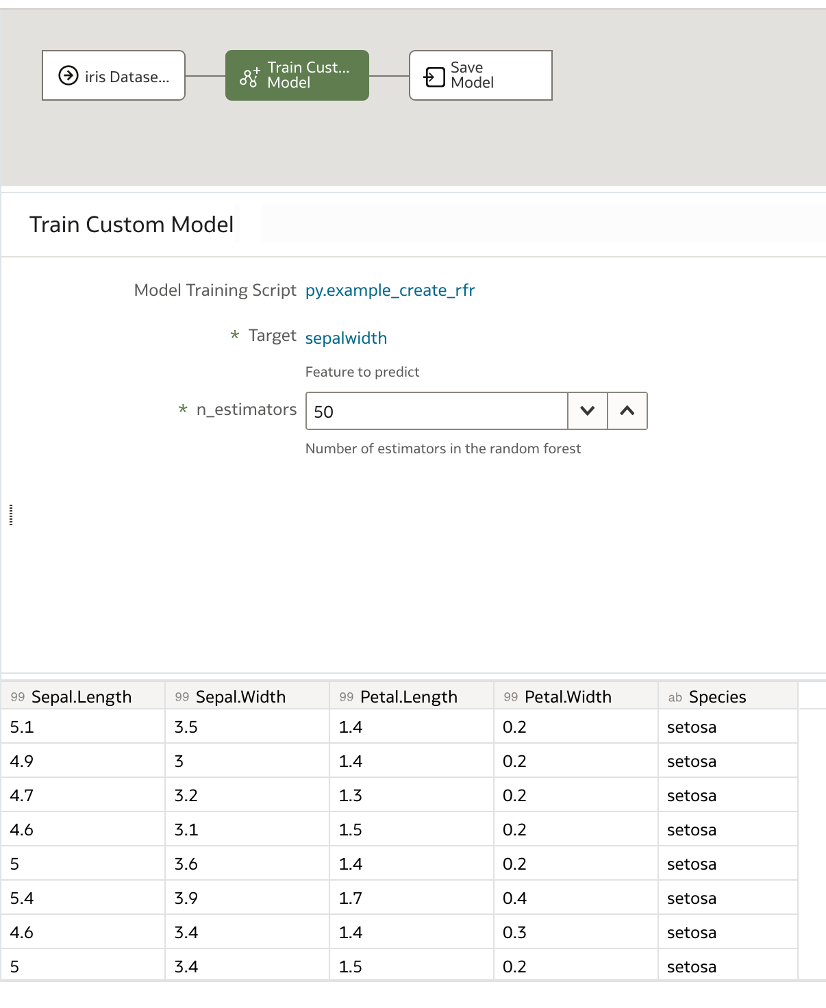
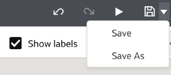
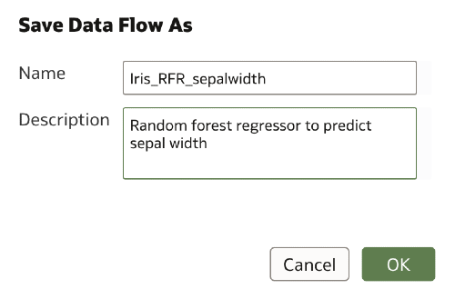
We specify our optional parameters, in our case the target and number of estimators, and finally name the output model before saving and running our data flow.

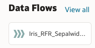
Once the data flow has finished, we can see our new model in the Home Screen.

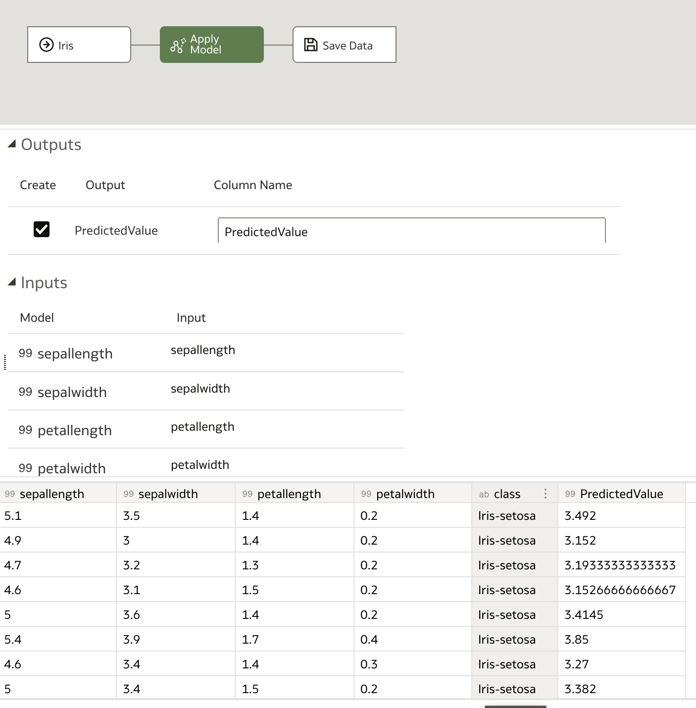
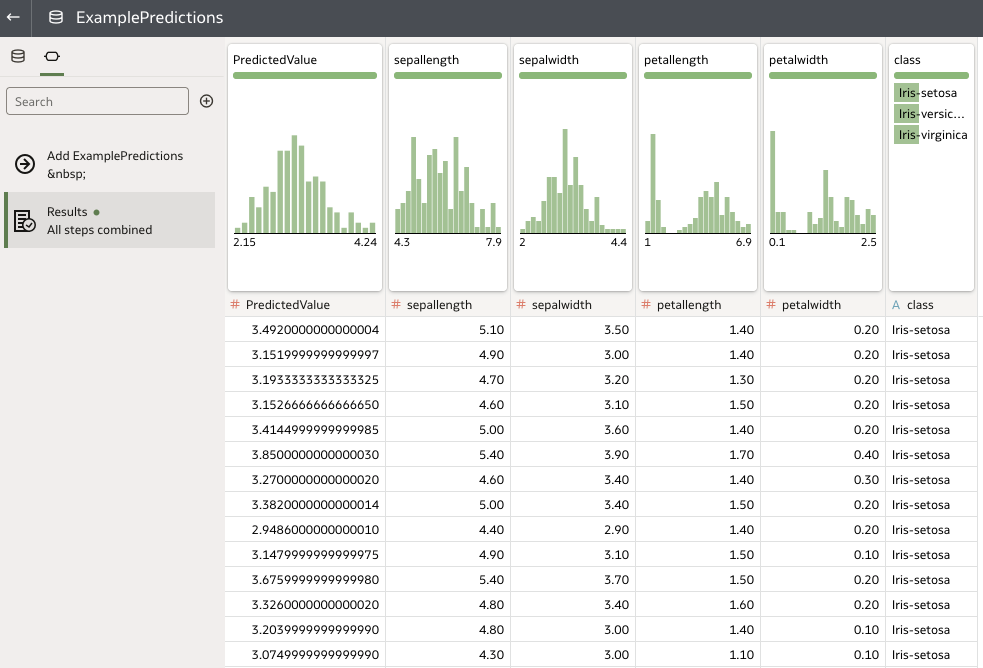
To apply the model, we once again click Create and then choose Data Flow. We choose our test dataset, and then add an Apply Model step. From the dropdown list, we can select our random forest regressor, and then see a preview of the dataset which will be generated.

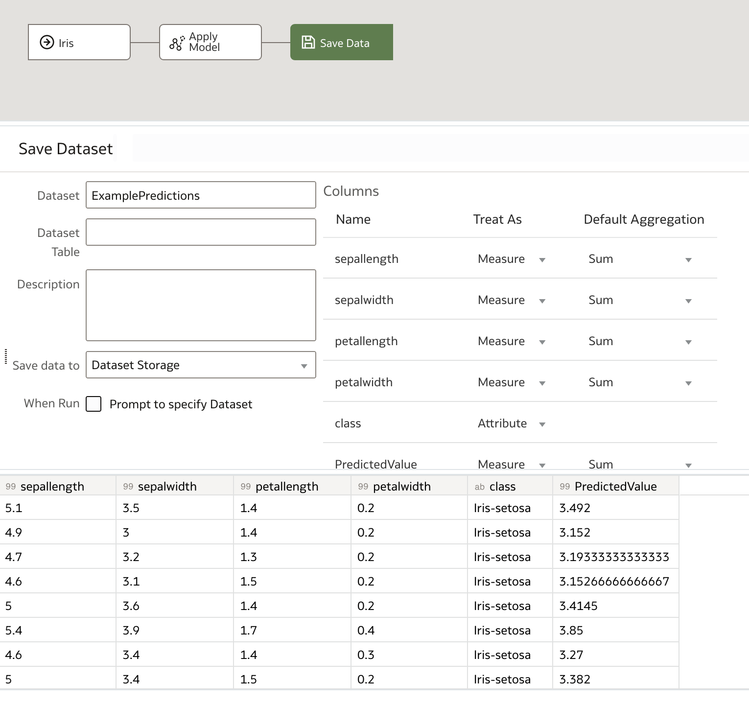
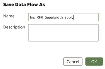
Finally, we save the output data, which contains our predictions and, optionally, the input dataset, name it as desired, and save it before running the data flow.

There we have it! Our set of predictions is now available to view or download. We are also free to re-apply our model to other input datasets and save their respective predictions separately using new data flows.

Rittman Mead Custom Tooling

There are a few pitfalls associated with embedding Python scripts into XML. For example, python code must be formatted correctly within scriptcontent XML field, there are static mandatory fields which must be populated, and files must be correctly titled for OAS to recognise them. Many of these requirements necessitate writing boilerplate code every time an XML is generated. Others require human understanding of the Python script (e.g. a working knowledge of the output columns and data types) and subsequent manual population of the XML file.

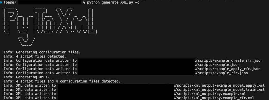
To facilitate this process and reduce manual effort in implementing custom scripts in OAS, Rittman Mead has developed Python-based script conversion tools which convert Python code with obi_execute_script, obi_create_modelor obi_apply_model functions to correctly formatted XML files. Our tooling can:

• Detect and correct incompatible comment formats
• Detect input arguments
• Embed Python scripts into XML files
• Automatically include mandatory boilerplate XML fields
• Automatically detect and unpack XML fields stored as metadata variables
• Automatically title apply_model and create_model scripts into correctly named pairs
• Highlight mandatory XML fields for which values cannot be automatically detected
• Generate JSON formatted config data to aid regeneration of XMLs

To find out more about how Rittman Mead can help with creating custom models in OAS, and for information on our other Data Science Services, please feel free to contact us at [email protected].